Mapping human lymph node cell types to 10X Visium with Cell2location
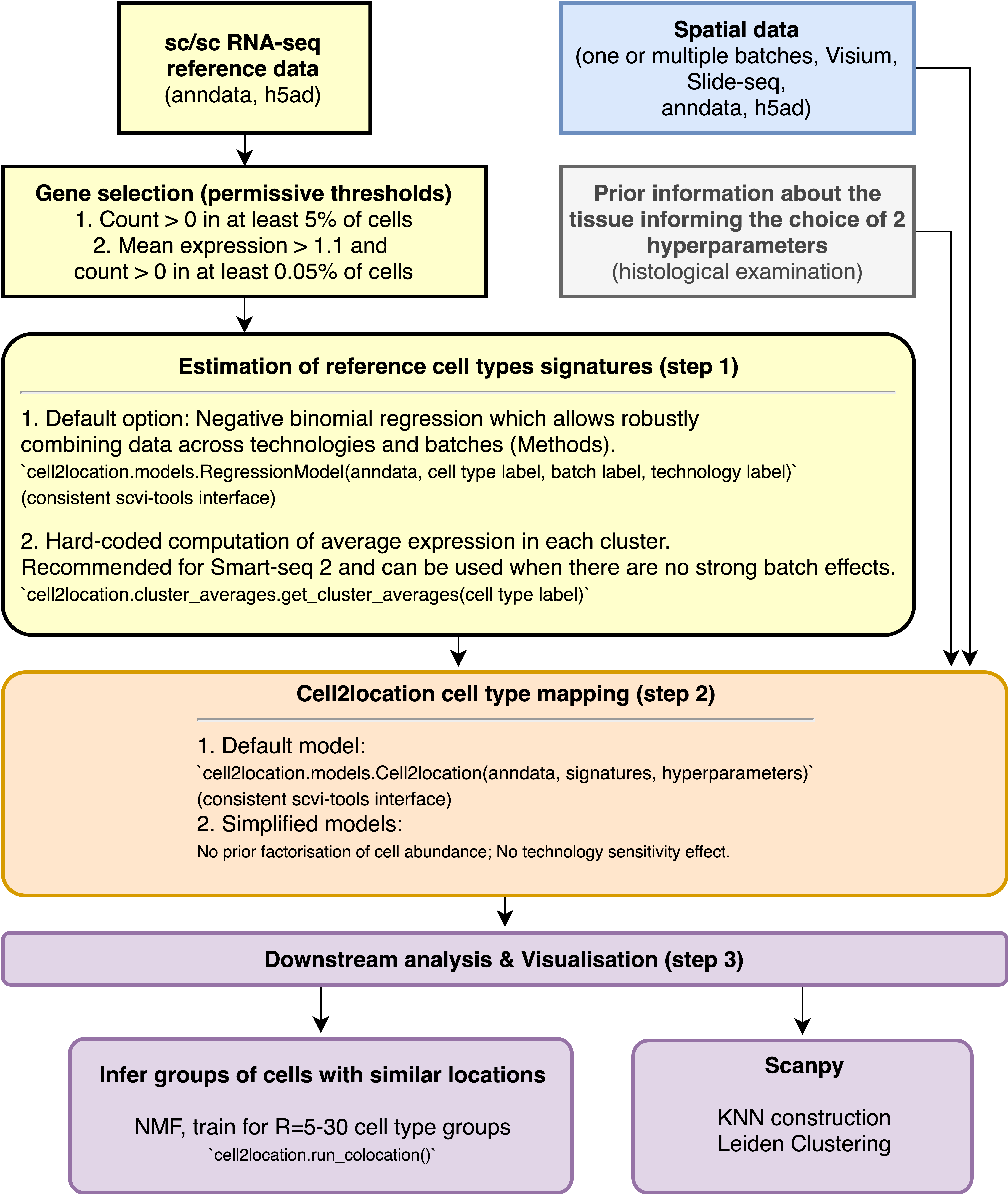
This tutorial shows how to use cell2location method for spatially resolving fine-grained cell types by integrating 10X Visium data with scRNA-seq reference of cell types. Cell2location is a principled Bayesian model that estimates which combination of cell types in which cell abundance could have given the mRNA counts in the spatial data, while modelling technical effects (platform/technology effect, contaminating RNA, unexplained variance).
Note!
Cell2location is an independent package, but is powered by scvi-tools. If you have questions about cell2location, Visium data or scvi-tools please visit https://discourse.scverse.org/c/ecosytem/cell2location/42, https://discourse.scverse.org/c/general/visium/32 or https://discourse.scverse.org/c/help/scvi-tools/7 correspondingly.
![]()
In this tutorial, we analyse a publicly available Visium dataset of the human lymph node from 10X Genomics, and spatially map a comprehensive atlas of 34 reference cell types derived by integration of scRNA-seq datasets from human secondary lymphoid organs.
Cell2location provides high sensitivity and resolution by borrowing statistical strength across locations. This is achieved by modelling similarity of location patterns between cell types using a hierarchical factorisation of cell abundance into tissue zones as a prior (see paper methods).
Using our statistical method based on Negative Binomial regression to robustly combine scRNA-seq reference data across technologies and batches results in improved spatial mapping accuracy. Given cell type annotation for each cell, the corresponding reference cell type signatures \(g_{f,g}\), which represent the average mRNA count of each gene \(g\) in each cell type \(f\), can be estimated from sc/snRNA-seq data using either 1) NB regression or 2) a hard-coded computation of per-cluster average mRNA counts for individual genes. We generally recommend using NB regression. This notebook shows use a dataset composed on multiple batches and technologies.When the batch effects are small, a faster hard-coded method of computing per cluster averages provides similarly high accuracy. We also recommend the hard-coded method for non-UMI technologies such as Smart-Seq 2.
Cell2location needs untransformed unnormalised spatial mRNA counts as input.
You also need to provide cell2location with the expected average cell abundance per location which is used as a prior to guide estimation of absolute cell abundance. This value depends on the tissue and can be estimated by counting nuclei for a few locations in the paired histology image but can be approximate (see paper methods for more guidance).
Workflow diagram
Contents
Loading packages
[1]:
import sys
IN_COLAB = "google.colab" in sys.modules
if IN_COLAB:
    !pip install --quiet scvi-colab
    from scvi_colab import install
    install()
    !pip install --quiet git+https://github.com/BayraktarLab/cell2location#egg=cell2location[tutorials]
[2]:
import scanpy as sc
import numpy as np
import matplotlib.pyplot as plt
import matplotlib as mpl

import cell2location

from matplotlib import rcParams
rcParams['pdf.fonttype'] = 42 # enables correct plotting of text for PDFs
Global seed set to 0
/nfs/team283/vk7/software/miniconda3farm5/envs/cell2loc_env2023/lib/python3.9/site-packages/pytorch_lightning/utilities/warnings.py:53: LightningDeprecationWarning: pytorch_lightning.utilities.warnings.rank_zero_deprecation has been deprecated in v1.6 and will be removed in v1.8. Use the equivalent function from the pytorch_lightning.utilities.rank_zero module instead.
  new_rank_zero_deprecation(
/nfs/team283/vk7/software/miniconda3farm5/envs/cell2loc_env2023/lib/python3.9/site-packages/pytorch_lightning/utilities/warnings.py:58: LightningDeprecationWarning: The `pytorch_lightning.loggers.base.rank_zero_experiment` is deprecated in v1.7 and will be removed in v1.9. Please use `pytorch_lightning.loggers.logger.rank_zero_experiment` instead.
  return new_rank_zero_deprecation(*args, **kwargs)
First, let’s define where we save the results of our analysis:
[3]:
results_folder = './results/lymph_nodes_analysis/'

# create paths and names to results folders for reference regression and cell2location models
ref_run_name = f'{results_folder}/reference_signatures'
run_name = f'{results_folder}/cell2location_map'
Loading Visium and scRNA-seq reference data
First let’s read spatial Visium data from 10X Space Ranger output. Here we use lymph node data generated by 10X and presented in Kleshchevnikov et al (section 4, Fig 4). This dataset can be conveniently downloaded and imported using scanpy. See this tutorial for a more extensive and practical example of data loading (multiple visium samples).
[4]:
adata_vis = sc.datasets.visium_sge(sample_id="V1_Human_Lymph_Node")
adata_vis.obs['sample'] = list(adata_vis.uns['spatial'].keys())[0]
/nfs/team283/vk7/software/miniconda3farm5/envs/cell2loc_env2023/lib/python3.9/site-packages/anndata/_core/anndata.py:1830: UserWarning: Variable names are not unique. To make them unique, call `.var_names_make_unique`.
  utils.warn_names_duplicates("var")
Note!
Here we rename genes to ENSEMBL ID for correct matching between single cell and spatial data - so you can ignore the scanpy suggestion to call .var_names_make_unique.
[5]:
adata_vis.var['SYMBOL'] = adata_vis.var_names
adata_vis.var.set_index('gene_ids', drop=True, inplace=True)
You can still plot gene expression by name using standard scanpy functions as follows:
sc.pl.spatial(color='PTPRC', gene_symbols='SYMBOL', ...)
Note!
Mitochondia-encoded genes (gene names start with prefix mt- or MT-) are irrelevant for spatial mapping because their expression represents technical artifacts in the single cell and nucleus data rather than biological abundance of mitochondria. Yet these genes compose 15-40% of mRNA in each location. Hence, to avoid mapping artifacts we strongly recommend removing mitochondrial genes.
[6]:
# find mitochondria-encoded (MT) genes
adata_vis.var['MT_gene'] = [gene.startswith('MT-') for gene in adata_vis.var['SYMBOL']]

# remove MT genes for spatial mapping (keeping their counts in the object)
adata_vis.obsm['MT'] = adata_vis[:, adata_vis.var['MT_gene'].values].X.toarray()
adata_vis = adata_vis[:, ~adata_vis.var['MT_gene'].values]
Published scRNA-seq datasets of lymph nodes have typically lacked an adequate representation of germinal centre-associated immune cell populations due to age of patient donors. We, therefore, include scRNA-seq datasets spanning lymph nodes, spleen and tonsils in our single-cell reference to ensure that we captured the full diversity of immune cell states likely to exist in the spatial transcriptomic dataset.
Here we download this dataset, import into anndata and change variable names to ENSEMBL gene identifiers.
[7]:
# Read data
adata_ref = sc.read(
    f'./data/sc.h5ad',
    backup_url='https://cell2location.cog.sanger.ac.uk/paper/integrated_lymphoid_organ_scrna/RegressionNBV4Torch_57covariates_73260cells_10237genes/sc.h5ad'
)
Warning
Here we rename genes to ENSEMBL ID for correct matching between single cell and spatial data.
[8]:
adata_ref.var['SYMBOL'] = adata_ref.var.index
# rename 'GeneID-2' as necessary for your data
adata_ref.var.set_index('GeneID-2', drop=True, inplace=True)

# delete unnecessary raw slot (to be removed in a future version of the tutorial)
del adata_ref.raw
Note!
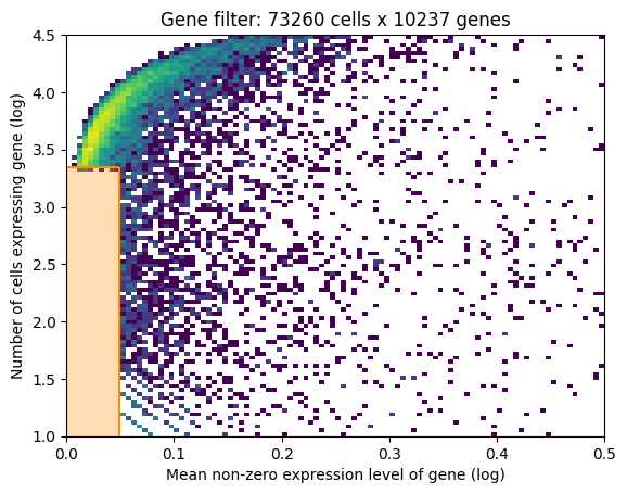
Before we estimate the reference cell type signature we recommend to perform very permissive genes selection. We prefer this to standard highly-variable-gene selection because our procedure keeps markers of rare genes while removing most of the uninformative genes.
The default parameters cell_count_cutoff=5, cell_percentage_cutoff2=0.03, nonz_mean_cutoff=1.12 are a good starting point, however, you can increase the cut-off to exclude more genes. To preserve marker genes of rare cell types we recommend low cell_count_cutoff=5, however, cell_percentage_cutoff2 and nonz_mean_cutoff can be increased to select between 8k-16k genes.
In this 2D histogram, orange rectangle highlights genes excluded based on the combination of number of cells expressing that gene (Y-axis) and average RNA count for cells where the gene was detected (X-axis).
In this case, the downloaded dataset was already filtered using this method, hence no density under the orange rectangle (to be changed in the future version of the tutorial).
[9]:
from cell2location.utils.filtering import filter_genes
selected = filter_genes(adata_ref, cell_count_cutoff=5, cell_percentage_cutoff2=0.03, nonz_mean_cutoff=1.12)

# filter the object
adata_ref = adata_ref[:, selected].copy()
Estimation of reference cell type signatures (NB regression)
The signatures are estimated from scRNA-seq data, accounting for batch effect, using a Negative binomial regression model.
[10]:
# prepare anndata for the regression model
cell2location.models.RegressionModel.setup_anndata(adata=adata_ref,
                        # 10X reaction / sample / batch
                        batch_key='Sample',
                        # cell type, covariate used for constructing signatures
                        labels_key='Subset',
                        # multiplicative technical effects (platform, 3' vs 5', donor effect)
                        categorical_covariate_keys=['Method']
                       )
No GPU/TPU found, falling back to CPU. (Set TF_CPP_MIN_LOG_LEVEL=0 and rerun for more info.)
[11]:
# create the regression model
from cell2location.models import RegressionModel
mod = RegressionModel(adata_ref)

# view anndata_setup as a sanity check
mod.view_anndata_setup()
Anndata setup with scvi-tools version 0.19.0.
Setup via `RegressionModel.setup_anndata` with arguments:
{
│   'layer': None,
│   'batch_key': 'Sample',
│   'labels_key': 'Subset',
│   'categorical_covariate_keys': ['Method'],
│   'continuous_covariate_keys': None
}
         Summary Statistics
┏━━━━━━━━━━━━━━━━━━━━━━━━━━┳━━━━━━━┓
┃     Summary Stat Key     ┃ Value ┃
┡━━━━━━━━━━━━━━━━━━━━━━━━━━╇━━━━━━━┩
│         n_batch          │  23   │
│         n_cells          │ 73260 │
│ n_extra_categorical_covs │   1   │
│ n_extra_continuous_covs  │   0   │
│         n_labels         │  34   │
│          n_vars          │ 10237 │
└──────────────────────────┴───────┘
                             Data Registry
┏━━━━━━━━━━━━━━━━━━━━━━━━┳━━━━━━━━━━━━━━━━━━━━━━━━━━━━━━━━━━━━━━━━━━━━┓
┃      Registry Key      ┃            scvi-tools Location             ┃
┡━━━━━━━━━━━━━━━━━━━━━━━━╇━━━━━━━━━━━━━━━━━━━━━━━━━━━━━━━━━━━━━━━━━━━━┩
│           X            │                  adata.X                   │
│         batch          │          adata.obs['_scvi_batch']          │
│ extra_categorical_covs │ adata.obsm['_scvi_extra_categorical_covs'] │
│         ind_x          │           adata.obs['_indices']            │
│         labels         │         adata.obs['_scvi_labels']          │
└────────────────────────┴────────────────────────────────────────────┘
                         batch State Registry
┏━━━━━━━━━━━━━━━━━━━━━┳━━━━━━━━━━━━━━━━━━━━━━━━┳━━━━━━━━━━━━━━━━━━━━━┓
┃   Source Location   ┃       Categories       ┃ scvi-tools Encoding ┃
┡━━━━━━━━━━━━━━━━━━━━━╇━━━━━━━━━━━━━━━━━━━━━━━━╇━━━━━━━━━━━━━━━━━━━━━┩
│ adata.obs['Sample'] │    4861STDY7135913     │          0          │
│                     │    4861STDY7135914     │          1          │
│                     │    4861STDY7208412     │          2          │
│                     │    4861STDY7208413     │          3          │
│                     │    4861STDY7462253     │          4          │
│                     │    4861STDY7462254     │          5          │
│                     │    4861STDY7462255     │          6          │
│                     │    4861STDY7462256     │          7          │
│                     │    4861STDY7528597     │          8          │
│                     │    4861STDY7528598     │          9          │
│                     │    4861STDY7528599     │         10          │
│                     │    4861STDY7528600     │         11          │
│                     │      BCP002_Total      │         12          │
│                     │      BCP003_Total      │         13          │
│                     │      BCP004_Total      │         14          │
│                     │      BCP005_Total      │         15          │
│                     │      BCP006_Total      │         16          │
│                     │      BCP008_Total      │         17          │
│                     │      BCP009_Total      │         18          │
│                     │ Human_colon_16S7255677 │         19          │
│                     │ Human_colon_16S7255678 │         20          │
│                     │ Human_colon_16S8000484 │         21          │
│                     │      Pan_T7935494      │         22          │
└─────────────────────┴────────────────────────┴─────────────────────┘
                     labels State Registry
┏━━━━━━━━━━━━━━━━━━━━━┳━━━━━━━━━━━━━━━━━━┳━━━━━━━━━━━━━━━━━━━━━┓
┃   Source Location   ┃    Categories    ┃ scvi-tools Encoding ┃
┡━━━━━━━━━━━━━━━━━━━━━╇━━━━━━━━━━━━━━━━━━╇━━━━━━━━━━━━━━━━━━━━━┩
│ adata.obs['Subset'] │    B_Cycling     │          0          │
│                     │     B_GC_DZ      │          1          │
│                     │     B_GC_LZ      │          2          │
│                     │    B_GC_prePB    │          3          │
│                     │      B_IFN       │          4          │
│                     │   B_activated    │          5          │
│                     │      B_mem       │          6          │
│                     │     B_naive      │          7          │
│                     │     B_plasma     │          8          │
│                     │     B_preGC      │          9          │
│                     │     DC_CCR7+     │         10          │
│                     │     DC_cDC1      │         11          │
│                     │     DC_cDC2      │         12          │
│                     │      DC_pDC      │         13          │
│                     │       Endo       │         14          │
│                     │       FDC        │         15          │
│                     │       ILC        │         16          │
│                     │  Macrophages_M1  │         17          │
│                     │  Macrophages_M2  │         18          │
│                     │       Mast       │         19          │
│                     │    Monocytes     │         20          │
│                     │        NK        │         21          │
│                     │       NKT        │         22          │
│                     │      T_CD4+      │         23          │
│                     │    T_CD4+_TfH    │         24          │
│                     │  T_CD4+_TfH_GC   │         25          │
│                     │   T_CD4+_naive   │         26          │
│                     │  T_CD8+_CD161+   │         27          │
│                     │ T_CD8+_cytotoxic │         28          │
│                     │   T_CD8+_naive   │         29          │
│                     │     T_TIM3+      │         30          │
│                     │      T_TfR       │         31          │
│                     │      T_Treg      │         32          │
│                     │       VSMC       │         33          │
└─────────────────────┴──────────────────┴─────────────────────┘
          extra_categorical_covs State Registry
┏━━━━━━━━━━━━━━━━━━━━━┳━━━━━━━━━━━━┳━━━━━━━━━━━━━━━━━━━━━┓
┃   Source Location   ┃ Categories ┃ scvi-tools Encoding ┃
┡━━━━━━━━━━━━━━━━━━━━━╇━━━━━━━━━━━━╇━━━━━━━━━━━━━━━━━━━━━┩
│ adata.obs['Method'] │    3GEX    │          0          │
│                     │    5GEX    │          1          │
│                     │            │                     │
└─────────────────────┴────────────┴─────────────────────┘
[12]:
mod.train(max_epochs=250, use_gpu=True)
GPU available: True (cuda), used: True
TPU available: False, using: 0 TPU cores
IPU available: False, using: 0 IPUs
HPU available: False, using: 0 HPUs
/nfs/team283/vk7/software/miniconda3farm5/envs/cell2loc_env2023/lib/python3.9/site-packages/pytorch_lightning/trainer/configuration_validator.py:105: UserWarning: You passed in a `val_dataloader` but have no `validation_step`. Skipping val loop.
  rank_zero_warn("You passed in a `val_dataloader` but have no `validation_step`. Skipping val loop.")
LOCAL_RANK: 0 - CUDA_VISIBLE_DEVICES: [0]
Epoch 250/250: 100%|█████████████████████████████████████████████████████████████████████████████████████████████| 250/250 [24:07<00:00, 5.76s/it, v_num=1, elbo_train=2.88e+8]
`Trainer.fit` stopped: `max_epochs=250` reached.
Epoch 250/250: 100%|█████████████████████████████████████████████████████████████████████████████████████████████| 250/250 [24:07<00:00, 5.79s/it, v_num=1, elbo_train=2.88e+8]
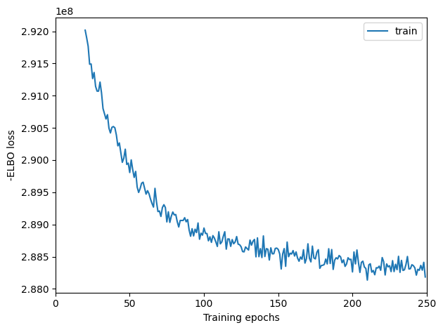
Here, we plot ELBO loss history during training, removing first 20 epochs from the plot. This plot should have a decreasing trend and level off by the end of training. If it is still decreasing, increase max_epochs.
[13]:
mod.plot_history(20)
[14]:
# In this section, we export the estimated cell abundance (summary of the posterior distribution).
adata_ref = mod.export_posterior(
    adata_ref, sample_kwargs={'num_samples': 1000, 'batch_size': 2500, 'use_gpu': True}
)

# Save model
mod.save(f"{ref_run_name}", overwrite=True)

# Save anndata object with results
adata_file = f"{ref_run_name}/sc.h5ad"
adata_ref.write(adata_file)
adata_file
Sampling local variables, batch:   0%|                                                                                                                   | 0/30 [00:00<?, ?it/s]
Sampling global variables, sample: 100%|██████████████████████████████████████████████████████████████████████████████████████████████████████| 999/999 [00:12<00:00, 82.46it/s]
[14]:
'./results/lymph_nodes_analysis//reference_signatures/sc.h5ad'
You can compute the 5%, 50% and 95% quantiles of the posterior distribution directly rather than using 1000 samples from the distribution (or any other quantiles). This speeds up application on large datasets and requires less memory - however, posterior mean and standard deviation cannot be computed this way.
adata_ref = mod.export_posterior(
    adata_ref, use_quantiles=True,
    # choose quantiles
    add_to_obsm=["q05","q50", "q95", "q0001"],
    sample_kwargs={'batch_size': 2500, 'use_gpu': True}
)
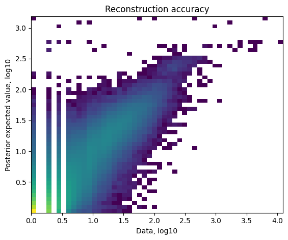
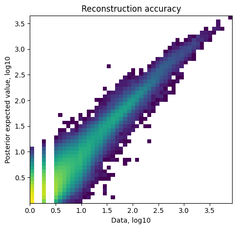
Reconstruction accuracy to assess if there are any issues with inference. This 2D histogram plot should have most observations along a noisy diagonal.
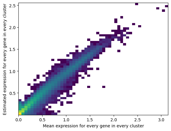
The estimated expression signatures are distinct from mean expression in each cluster because of batch effects. For scRNA-seq datasets which do not suffer from batch effect (this dataset does), cluster average expression can be used instead of estimating signatures with a model. When this plot is very different from a diagonal plot (e.g. very low values on Y-axis, density everywhere) it indicates problems with signature estimation.
[15]:
mod.plot_QC()
The model and output h5ad can be loaded later like this:
adata_file = f"{ref_run_name}/sc.h5ad"
adata_ref = sc.read_h5ad(adata_file)
mod = cell2location.models.RegressionModel.load(f"{ref_run_name}", adata_ref)
[16]:
# export estimated expression in each cluster
if 'means_per_cluster_mu_fg' in adata_ref.varm.keys():
    inf_aver = adata_ref.varm['means_per_cluster_mu_fg'][[f'means_per_cluster_mu_fg_{i}'
                                    for i in adata_ref.uns['mod']['factor_names']]].copy()
else:
    inf_aver = adata_ref.var[[f'means_per_cluster_mu_fg_{i}'
                                    for i in adata_ref.uns['mod']['factor_names']]].copy()
inf_aver.columns = adata_ref.uns['mod']['factor_names']
inf_aver.iloc[0:5, 0:5]
[16]:
| B_Cycling | B_GC_DZ | B_GC_LZ | B_GC_prePB | B_IFN | |
|---|---|---|---|---|---|
| GeneID-2 | |||||
| ENSG00000188976 | 0.432963 | 0.244077 | 0.311908 | 0.350530 | 0.152206 |
| ENSG00000188290 | 0.002115 | 0.000746 | 0.000777 | 0.057073 | 0.040800 |
| ENSG00000187608 | 0.385745 | 0.212942 | 0.275868 | 0.513321 | 3.958895 |
| ENSG00000186891 | 0.019910 | 0.000785 | 0.055453 | 0.069395 | 0.011100 |
| ENSG00000186827 | 0.007769 | 0.000548 | 0.006403 | 0.030153 | 0.011449 |
Cell2location: spatial mapping
[17]:
# find shared genes and subset both anndata and reference signatures
intersect = np.intersect1d(adata_vis.var_names, inf_aver.index)
adata_vis = adata_vis[:, intersect].copy()
inf_aver = inf_aver.loc[intersect, :].copy()

# prepare anndata for cell2location model
cell2location.models.Cell2location.setup_anndata(adata=adata_vis, batch_key="sample")
To use cell2location spatial mapping model, you need to specify 2 user-provided hyperparameters (N_cells_per_location and detection_alpha) - for detailed guidance on setting these hyperparameters and their impact see the flow diagram and the note.
Choosing hyperparameter ``N_cells_per_location``!
It is useful to adapt the expected cell abundance N_cells_per_location to every tissue. This value can be estimated from paired histology images and as described in the note above. Change the value presented in this tutorial (N_cells_per_location=30) to the value observed in your your tissue.
Choosing hyperparameter ``detection_alpha``!
To improve accuracy & sensitivity on datasets with large technical variability in RNA detection sensitivity within the slide/batch - you need to relax regularisation of per-location normalisation (use detection_alpha=20). High technical variability in RNA detection sensitivity is present in your sample when you observe the spatial distribution of total RNA count per location that doesn’t match expected cell numbers based on histological examination.
We initially opted for high regularisation (detection_alpha=200) as a default because the mouse brain & human lymph node datasets used in our paper have low technical effects and using high regularisation strenght improves consistencly between total estimated cell abundance per location and the nuclei count quantified from histology (Fig S8F in cell2location paper).
However, in many collaborations, we see that Visium experiments on human tissues suffer from technical effects. This motivates the new default value of detection_alpha=20 and the recommendation of testing both settings on your data (detection_alpha=20 and detection_alpha=200).
[18]:
# create and train the model
mod = cell2location.models.Cell2location(
    adata_vis, cell_state_df=inf_aver,
    # the expected average cell abundance: tissue-dependent
    # hyper-prior which can be estimated from paired histology:
    N_cells_per_location=30,
    # hyperparameter controlling normalisation of
    # within-experiment variation in RNA detection:
    detection_alpha=20
)
mod.view_anndata_setup()
Anndata setup with scvi-tools version 0.19.0.
Setup via `Cell2location.setup_anndata` with arguments:
{
│   'layer': None,
│   'batch_key': 'sample',
│   'labels_key': None,
│   'categorical_covariate_keys': None,
│   'continuous_covariate_keys': None
}
         Summary Statistics
┏━━━━━━━━━━━━━━━━━━━━━━━━━━┳━━━━━━━┓
┃     Summary Stat Key     ┃ Value ┃
┡━━━━━━━━━━━━━━━━━━━━━━━━━━╇━━━━━━━┩
│         n_batch          │   1   │
│         n_cells          │ 4035  │
│ n_extra_categorical_covs │   0   │
│ n_extra_continuous_covs  │   0   │
│         n_labels         │   1   │
│          n_vars          │ 10217 │
└──────────────────────────┴───────┘
               Data Registry
┏━━━━━━━━━━━━━━┳━━━━━━━━━━━━━━━━━━━━━━━━━━━┓
┃ Registry Key ┃    scvi-tools Location    ┃
┡━━━━━━━━━━━━━━╇━━━━━━━━━━━━━━━━━━━━━━━━━━━┩
│      X       │          adata.X          │
│    batch     │ adata.obs['_scvi_batch']  │
│    ind_x     │   adata.obs['_indices']   │
│    labels    │ adata.obs['_scvi_labels'] │
└──────────────┴───────────────────────────┘
                       batch State Registry
┏━━━━━━━━━━━━━━━━━━━━━┳━━━━━━━━━━━━━━━━━━━━━┳━━━━━━━━━━━━━━━━━━━━━┓
┃   Source Location   ┃     Categories      ┃ scvi-tools Encoding ┃
┡━━━━━━━━━━━━━━━━━━━━━╇━━━━━━━━━━━━━━━━━━━━━╇━━━━━━━━━━━━━━━━━━━━━┩
│ adata.obs['sample'] │ V1_Human_Lymph_Node │          0          │
└─────────────────────┴─────────────────────┴─────────────────────┘
                     labels State Registry
┏━━━━━━━━━━━━━━━━━━━━━━━━━━━┳━━━━━━━━━━━━┳━━━━━━━━━━━━━━━━━━━━━┓
┃      Source Location      ┃ Categories ┃ scvi-tools Encoding ┃
┡━━━━━━━━━━━━━━━━━━━━━━━━━━━╇━━━━━━━━━━━━╇━━━━━━━━━━━━━━━━━━━━━┩
│ adata.obs['_scvi_labels'] │     0      │          0          │
└───────────────────────────┴────────────┴─────────────────────┘
[19]:
mod.train(max_epochs=30000,
# train using full data (batch_size=None)
batch_size=None,
# use all data points in training because
# we need to estimate cell abundance at all locations
train_size=1,
use_gpu=True,
)
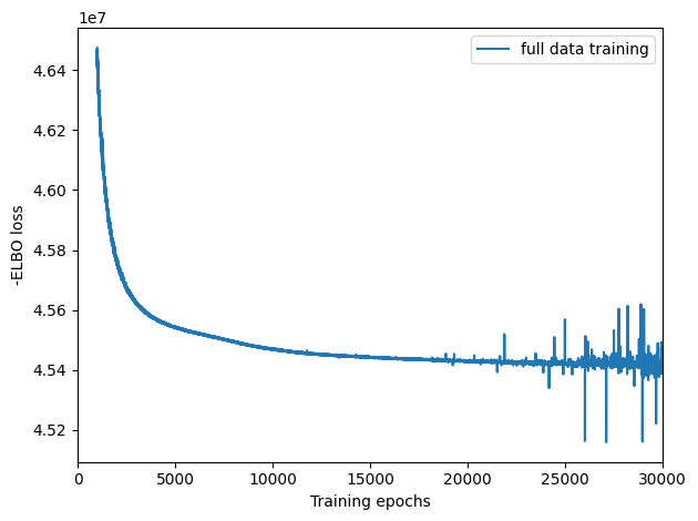
# plot ELBO loss history during training, removing first 100 epochs from the plot
mod.plot_history(1000)
plt.legend(labels=['full data training']);
GPU available: True (cuda), used: True
TPU available: False, using: 0 TPU cores
IPU available: False, using: 0 IPUs
HPU available: False, using: 0 HPUs
/nfs/team283/vk7/software/miniconda3farm5/envs/cell2loc_env2023/lib/python3.9/site-packages/pytorch_lightning/trainer/configuration_validator.py:105: UserWarning: You passed in a `val_dataloader` but have no `validation_step`. Skipping val loop.
  rank_zero_warn("You passed in a `val_dataloader` but have no `validation_step`. Skipping val loop.")
LOCAL_RANK: 0 - CUDA_VISIBLE_DEVICES: [0]
/nfs/team283/vk7/software/miniconda3farm5/envs/cell2loc_env2023/lib/python3.9/site-packages/pytorch_lightning/trainer/trainer.py:1892: PossibleUserWarning: The number of training batches (1) is smaller than the logging interval Trainer(log_every_n_steps=10). Set a lower value for log_every_n_steps if you want to see logs for the training epoch.
  rank_zero_warn(
Epoch 30000/30000: 100%|█████████████████████████████████████████████████████████████████████████████████████| 30000/30000 [45:40<00:00, 10.91it/s, v_num=1, elbo_train=4.54e+7]
`Trainer.fit` stopped: `max_epochs=30000` reached.
Epoch 30000/30000: 100%|█████████████████████████████████████████████████████████████████████████████████████| 30000/30000 [45:40<00:00, 10.95it/s, v_num=1, elbo_train=4.54e+7]
[20]:
# In this section, we export the estimated cell abundance (summary of the posterior distribution).
adata_vis = mod.export_posterior(
    adata_vis, sample_kwargs={'num_samples': 1000, 'batch_size': mod.adata.n_obs, 'use_gpu': True}
)

# Save model
mod.save(f"{run_name}", overwrite=True)

# mod = cell2location.models.Cell2location.load(f"{run_name}", adata_vis)

# Save anndata object with results
adata_file = f"{run_name}/sp.h5ad"
adata_vis.write(adata_file)
adata_file
Sampling local variables, batch: 100%|████████████████████████████████████████████████████████████████████████████████████████████████████████████| 1/1 [00:18<00:00, 18.21s/it]
Sampling global variables, sample: 100%|██████████████████████████████████████████████████████████████████████████████████████████████████████| 999/999 [00:19<00:00, 51.98it/s]
[20]:
'./results/lymph_nodes_analysis//cell2location_map/sp.h5ad'
The model and output h5ad can be loaded later like this:
adata_file = f"{run_name}/sp.h5ad"
adata_vis = sc.read_h5ad(adata_file)
mod = cell2location.models.Cell2location.load(f"{run_name}", adata_vis)
[21]:
mod.plot_QC()
When intergrating multiple spatial batches and when working with datasets that have substantial variation of detected RNA within slides (that cannot be explained by high cellular density in the histology), it is important to assess whether cell2location normalised those effects. You expect to see similar total cell abundance across batches but distinct RNA detection sensitivity (both estimated by cell2location). You expect total cell abundance to mirror high cellular density in the histology.
fig = mod.plot_spatial_QC_across_batches()
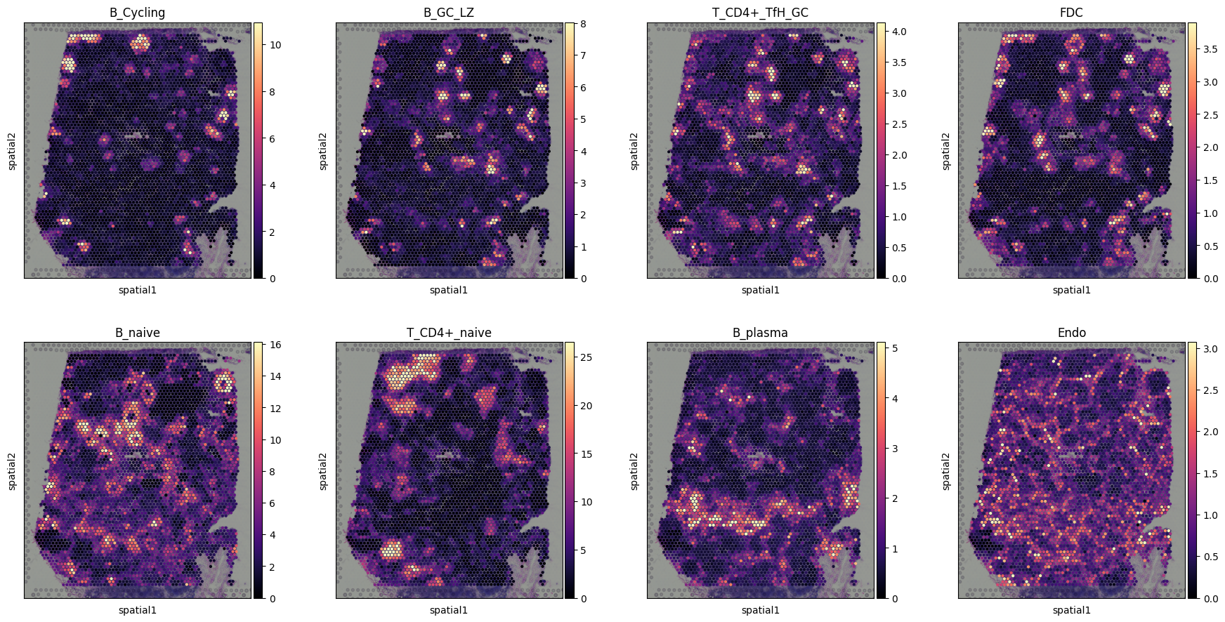
Visualising cell abundance in spatial coordinates
Note
We use 5% quantile of the posterior distribution, representing the value of cell abundance that the model has high confidence in (aka ‘at least this amount is present’).
[22]:
# add 5% quantile, representing confident cell abundance, 'at least this amount is present',
# to adata.obs with nice names for plotting
adata_vis.obs[adata_vis.uns['mod']['factor_names']] = adata_vis.obsm['q05_cell_abundance_w_sf']

# select one slide
from cell2location.utils import select_slide
slide = select_slide(adata_vis, 'V1_Human_Lymph_Node')

# plot in spatial coordinates
with mpl.rc_context({'axes.facecolor':  'black',
                     'figure.figsize': [4.5, 5]}):

    sc.pl.spatial(slide, cmap='magma',
                  # show first 8 cell types
                  color=['B_Cycling', 'B_GC_LZ', 'T_CD4+_TfH_GC', 'FDC',
                         'B_naive', 'T_CD4+_naive', 'B_plasma', 'Endo'],
                  ncols=4, size=1.3,
                  img_key='hires',
                  # limit color scale at 99.2% quantile of cell abundance
                  vmin=0, vmax='p99.2'
                 )
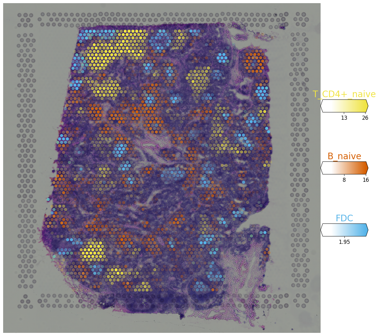
[23]:
# Now we use cell2location plotter that allows showing multiple cell types in one panel
from cell2location.plt import plot_spatial

# select up to 6 clusters
clust_labels = ['T_CD4+_naive', 'B_naive', 'FDC']
clust_col = ['' + str(i) for i in clust_labels] # in case column names differ from labels

slide = select_slide(adata_vis, 'V1_Human_Lymph_Node')

with mpl.rc_context({'figure.figsize': (15, 15)}):
    fig = plot_spatial(
        adata=slide,
        # labels to show on a plot
        color=clust_col, labels=clust_labels,
        show_img=True,
        # 'fast' (white background) or 'dark_background'
        style='fast',
        # limit color scale at 99.2% quantile of cell abundance
        max_color_quantile=0.992,
        # size of locations (adjust depending on figure size)
        circle_diameter=6,
        colorbar_position='right'
    )
Downstream analysis
Identifying discrete tissue regions by Leiden clustering
We identify tissue regions that differ in their cell composition by clustering locations using cell abundance estimated by cell2location.
We find tissue regions by clustering Visium spots using estimated cell abundance each cell type. We constuct a K-nearest neigbour (KNN) graph representing similarity of locations in estimated cell abundance and then apply Leiden clustering. The number of KNN neighbours should be adapted to size of dataset and the size of anatomically defined regions (e.i. hippocampus regions are rather small compared to size of the brain so could be masked by large n_neighbors). This can be done for a range
KNN neighbours and Leiden clustering resolutions until a clustering matching the anatomical structure of the tissue is obtained.
The clustering is done jointly across all Visium sections / batches, hence the region identities are directly comparable. When there are strong technical effects between multiple batches (not the case here) sc.external.pp.bbknn can be in principle used to account for those effects during the KNN construction.
The resulting clusters are saved in adata_vis.obs['region_cluster'].
[24]:
# compute KNN using the cell2location output stored in adata.obsm
sc.pp.neighbors(adata_vis, use_rep='q05_cell_abundance_w_sf',
                n_neighbors = 15)

# Cluster spots into regions using scanpy
sc.tl.leiden(adata_vis, resolution=1.1)

# add region as categorical variable
adata_vis.obs["region_cluster"] = adata_vis.obs["leiden"].astype("category")
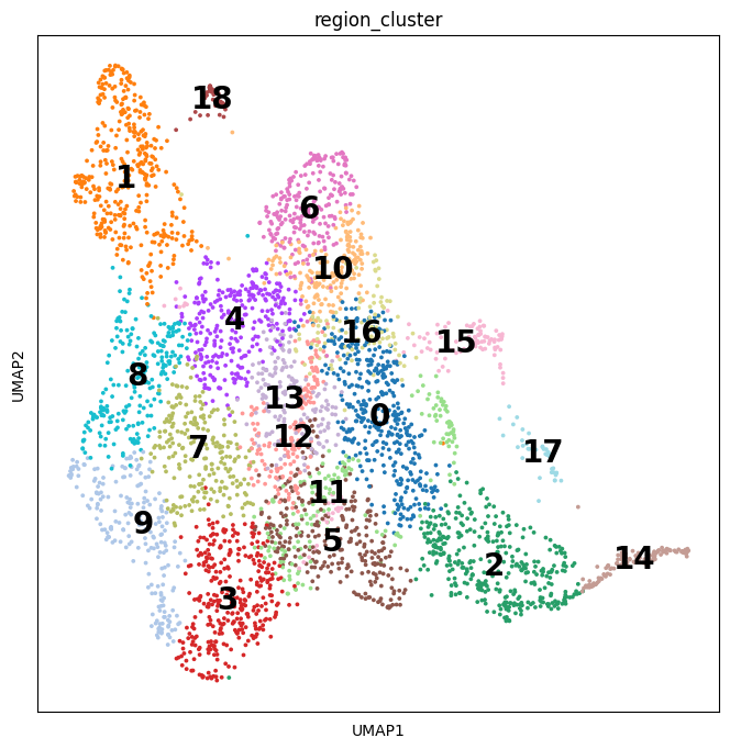
We can use the location composition similarity graph to build a joint integrated UMAP representation of all section/Visium batches.
[25]:
# compute UMAP using KNN graph based on the cell2location output
sc.tl.umap(adata_vis, min_dist = 0.3, spread = 1)
# show regions in UMAP coordinates
with mpl.rc_context({'axes.facecolor': 'white',
'figure.figsize': [8, 8]}):
sc.pl.umap(adata_vis, color=['region_cluster'], size=30,
color_map = 'RdPu', ncols = 2, legend_loc='on data',
legend_fontsize=20)
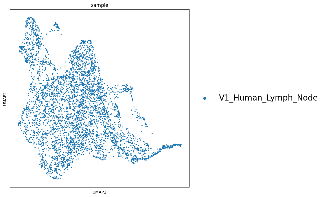
sc.pl.umap(adata_vis, color=['sample'], size=30,
color_map = 'RdPu', ncols = 2,
legend_fontsize=20)
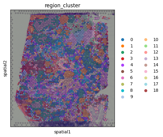
# plot in spatial coordinates
with mpl.rc_context({'axes.facecolor': 'black',
'figure.figsize': [4.5, 5]}):
sc.pl.spatial(adata_vis, color=['region_cluster'],
size=1.3, img_key='hires', alpha=0.5)
/nfs/team283/vk7/software/miniconda3farm5/envs/cell2loc_env2023/lib/python3.9/site-packages/scanpy/plotting/_tools/scatterplots.py:392: UserWarning: No data for colormapping provided via 'c'. Parameters 'cmap' will be ignored
  cax = scatter(
/nfs/team283/vk7/software/miniconda3farm5/envs/cell2loc_env2023/lib/python3.9/site-packages/scanpy/plotting/_tools/scatterplots.py:392: UserWarning: No data for colormapping provided via 'c'. Parameters 'cmap' will be ignored
  cax = scatter(
Identifying cellular compartments / tissue zones using matrix factorisation (NMF)
Here, we use the cell2location mapping results to identify the spatial co-occurrence of cell types in order to better understand the tissue organisation and predict cellular interactions. We performed non-negative matrix factorization (NMF) of the cell type abundance estimates from cell2location (paper section 4, Fig 4D). Similar to the established benefits of applying NMF to conventional scRNA-seq, the additive NMF decomposition yielded a grouping of spatial cell type abundance profiles into components that capture co-localised cell types (Supplemenary Methods section 4.2, p. 60). This NMF-based decomposition naturally accounts for the fact that multiple cell types and microenvironments can co-exist at the same Visium locations (see paper Fig S20, p. 34), while sharing information across tissue areas (e.g. individual germinal centres).
Tip
In practice, it is better to train NMF for a range of factors \(R={5, .., 30}\) and select \(R\) as a balance between capturing fine-grained and splitting known well-established tissue zones.
If you want to find a few most disctinct cellular compartments, use a small number of factors. If you want to find very strong co-location signal and assume that most cell types don’t co-locate, use a lot of factors (> 30 - used here).
Below we show how to perform this analysis. To aid this analysis, we wrapped the analysis shown the notebook on advanced downstream analysis into a pipeline that automates training of the NMF model with varying number of factors:
[26]:
from cell2location import run_colocation
res_dict, adata_vis = run_colocation(
    adata_vis,
    model_name='CoLocatedGroupsSklearnNMF',
    train_args={
      'n_fact': np.arange(11, 13), # IMPORTANT: use a wider range of the number of factors (5-30)
      'sample_name_col': 'sample', # columns in adata_vis.obs that identifies sample
      'n_restarts': 3 # number of training restarts
    },
    # the hyperparameters of NMF can be also adjusted:
    model_kwargs={'alpha': 0.01, 'init': 'random', "nmf_kwd_args": {"tol": 0.000001}},
    export_args={'path': f'{run_name}/CoLocatedComb/'}
)
### Analysis name: CoLocatedGroupsSklearnNMF_11combinations_4035locations_34factors
WARNING: saving figure to file results/lymph_nodes_analysis/cell2location_map/CoLocatedComb/CoLocatedGroupsSklearnNMF_4035locations_34factors/spatial/showcell_density_mean_n_fact11_sV1_Human_Lymph_Node_p99.2.pdf
### Analysis name: CoLocatedGroupsSklearnNMF_12combinations_4035locations_34factors
WARNING: saving figure to file results/lymph_nodes_analysis/cell2location_map/CoLocatedComb/CoLocatedGroupsSklearnNMF_4035locations_34factors/spatial/showcell_density_mean_n_fact12_sV1_Human_Lymph_Node_p99.2.pdf
For every factor number, the model produces the following list of folder outputs:
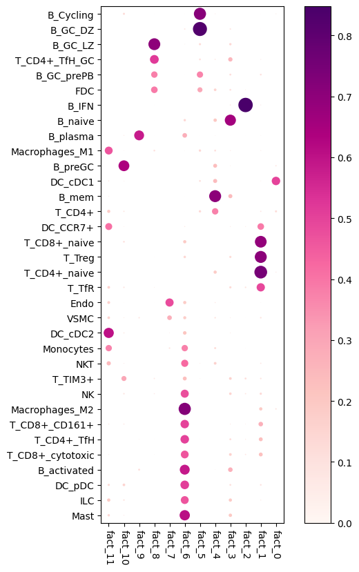
cell_type_fractions_heatmap/: a dot plot of the estimated NMF weights of cell types (rows) across NMF components (columns)
cell_type_fractions_mean/: the data used for dot plot
factor_markers/: tables listing top 10 cell types most speficic to each NMF factor
models/: saved NMF models
predictive_accuracy/: 2D histogram plot showing how well NMF explains cell2location output
spatial/: NMF weights across locatinos in spatial coordinates
location_factors_mean/: the data used for the plot in spatial coordiantes
stability_plots/: stability of NMF weights between training restarts
Key output that you want to examine are the files in cell_type_fractions_heatmap/ which show a dot plot of the estimated NMF weights of cell types (rows) across NMF components (columns) which correspond to cellular compartments. Shown are relative weights, normalized across components for every cell type.
Tip
The NMF model output such as factor loadings are stored in adata.uns[f"mod_coloc_n_fact{n_fact}"] in a similar output format as main cell2location results in adata.uns['mod'].
[27]:
# Here we plot the NMF weights (Same as saved to `cell_type_fractions_heatmap`)
res_dict['n_fact12']['mod'].plot_cell_type_loadings()
Estimate cell-type specific expression of every gene in the spatial data (needed for NCEM)
The cell-type specific expression of every gene at every spatial location in the spatial data enables learning cell communication with NCEM model using Visium data (https://github.com/theislab/ncem).
To derive this, we adapt the approach of estimating conditional expected expression proposed by RCTD (Cable et al) method.
With cell2location, we can look at the posterior distribution rather than just point estimates of cell type specific expression (see mod.samples.keys() and next section on using full distribution).
Note that this analysis requires substantial amount of RAM memory and thefore doesn’t work on free Google Colab (12 GB limit).
[28]:
# Compute expected expression per cell type
expected_dict = mod.module.model.compute_expected_per_cell_type(
    mod.samples["post_sample_q05"], mod.adata_manager
)

# Add to anndata layers
for i, n in enumerate(mod.factor_names_):
    adata_vis.layers[n] = expected_dict['mu'][i]

# Save anndata object with results
adata_file = f"{run_name}/sp.h5ad"
adata_vis.write(adata_file)
adata_file
[28]:
'./results/lymph_nodes_analysis//cell2location_map/sp.h5ad'
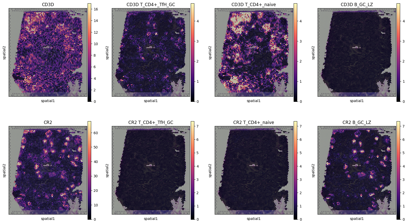
Plotting cell-type specific expression of genes in spatial coordinates.
Below we plot the cell-type specific expression of genes (rows, second to last columns) compared to total expression of those genes (first column).
Here we highlight CD3D, pan T-cell marker expressed by 2 subtypes of T cells in distinct locations but not expressed by co-located B cells, that instead express CR2 gene.
[29]:
# list cell types and genes for plotting
ctypes = ['T_CD4+_TfH_GC', 'T_CD4+_naive', 'B_GC_LZ']
genes = ['CD3D', 'CR2']

with mpl.rc_context({'axes.facecolor':  'black'}):
    # select one slide
    slide = select_slide(adata_vis, 'V1_Human_Lymph_Node')

    from tutorial_utils import plot_genes_per_cell_type
    plot_genes_per_cell_type(slide, genes, ctypes);
Note that plot_genes_per_cell_type function often need customization so it is not included into cell2location package - you need to copy it from https://github.com/BayraktarLab/cell2location/blob/master/docs/notebooks/tutorial_utils.py to use on your system.
Advanced use
Working with the posterior distribution and computing arbitrary quantiles
In addition to the posterior distribution mean, std and quantiles presented earlier in the notebook you can fetch an arbitrary number of samples from the posterior distribution. To limit memory use, it could be beneficial to select particular varibles in the model.
Note that this analysis requires substantial amount RAM memory and thefore doesn’t work on Google Colab.
[30]:
# Get posterior distribution samples for specific variables
samples_w_sf = mod.sample_posterior(num_samples=1000, use_gpu=True, return_samples=True,
                                    batch_size=2020,
                                    return_sites=['w_sf', 'm_g', 'u_sf_mRNA_factors'])
# samples_w_sf['posterior_samples'] contains 1000 samples as arrays with dim=(num_samples, ...)
samples_w_sf['posterior_samples']['w_sf'].shape
Sampling local variables, batch: 100%|████████████████████████████████████████████████████████████████████████████████████████████████████████████| 2/2 [00:29<00:00, 14.61s/it]
Sampling global variables, sample: 100%|██████████████████████████████████████████████████████████████████████████████████████████████████████| 999/999 [00:15<00:00, 63.04it/s]
[30]:
(1000, 4035, 34)
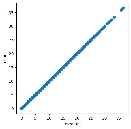
Finally, it could be useful to compute arbitrary quantiles of the posterior distribution.
[31]:
# Compute any quantile of the posterior distribution
medians = mod.posterior_quantile(q=0.5, batch_size=mod.adata.n_obs, use_gpu=True)

with mpl.rc_context({'axes.facecolor':  'white',
                     'figure.figsize': [5, 5]}):
    plt.scatter(medians['w_sf'].flatten(), mod.samples['post_sample_means']['w_sf'].flatten());
    plt.xlabel('median');
    plt.ylabel('mean');
Modules and their versions used for this analysis
Useful for debugging and reporting issues.
[32]:
cell2location.utils.list_imported_modules()
sys 3.9.16 (main, Jan 11 2023, 16:05:54)
[GCC 11.2.0]
re 2.2.1
ipykernel._version 6.20.2
json 2.0.9
jupyter_client._version 7.4.9
traitlets._version 5.8.1
traitlets 5.8.1
logging 0.5.1.2
platform 1.0.8
_ctypes 1.1.0
ctypes 1.1.0
zmq.sugar.version 25.0.0
zmq.sugar 25.0.0
zmq 25.0.0
tornado 6.2
zlib 1.0
_curses b'2.2'
socketserver 0.4
argparse 1.1
dateutil._version 2.8.2
dateutil 2.8.2
six 1.16.0
_decimal 1.70
decimal 1.70
jupyter_core.version 5.1.5
jupyter_core 5.1.5
platformdirs.version 2.6.2
platformdirs 2.6.2
entrypoints 0.4
jupyter_client 7.4.9
ipykernel 6.20.2
IPython.core.release 8.8.0
executing.version 1.2.0
executing 1.2.0
pure_eval.version 0.2.2
pure_eval 0.2.2
stack_data.version 0.6.2
stack_data 0.6.2
pygments 2.14.0
ptyprocess 0.7.0
pexpect 4.8.0
IPython.core.crashhandler 8.8.0
pickleshare 0.7.5
backcall 0.2.0
decorator 5.1.1
_sqlite3 2.6.0
sqlite3.dbapi2 2.6.0
sqlite3 2.6.0
wcwidth 0.2.6
prompt_toolkit 3.0.36
parso 0.8.3
jedi 0.18.2
urllib.request 3.9
IPython.core.magics.code 8.8.0
IPython 8.8.0
comm 0.1.2
psutil 5.9.4
debugpy.public_api 1.6.6
debugpy 1.6.6
xmlrpc.client 3.9
http.server 0.6
pkg_resources._vendor.more_itertools 8.12.0
pkg_resources.extern.more_itertools 8.12.0
pkg_resources._vendor.appdirs 1.4.3
pkg_resources.extern.appdirs 1.4.3
pkg_resources._vendor.packaging.__about__ 21.3
pkg_resources._vendor.packaging 21.3
pkg_resources.extern.packaging 21.3
pkg_resources._vendor.pyparsing 3.0.9
pkg_resources.extern.pyparsing 3.0.9
_pydevd_frame_eval.vendored.bytecode 0.13.0.dev
_pydev_bundle.fsnotify 0.1.5
pydevd 2.9.5
packaging 23.0
_csv 1.0
csv 1.0
scanpy._metadata 1.9.1
numpy.version 1.23.5
numpy.core._multiarray_umath 3.1
numpy.core 1.23.5
numpy.linalg._umath_linalg 0.1.5
numpy.lib 1.23.5
numpy 1.23.5
scipy.version 1.10.0
scipy 1.10.0
scipy.sparse.linalg._isolve._iterative b'$Revision: $'
scipy._lib.decorator 4.0.5
scipy.linalg._fblas b'$Revision: $'
scipy.linalg._flapack b'$Revision: $'
scipy.linalg._flinalg b'$Revision: $'
scipy.sparse.linalg._eigen.arpack._arpack b'$Revision: $'
anndata._metadata 0.8.0
h5py.version 3.8.0
h5py 3.8.0
natsort 8.2.0
pytz 2022.7.1
tarfile 0.9.0
pandas 1.5.3
anndata 0.8.0
yaml 6.0
llvmlite 0.39.1
numba.cloudpickle 1.6.0
numba.misc.appdirs 1.4.1
numba 0.56.4
setuptools._distutils 3.9.16
setuptools.version 65.6.3
setuptools._vendor.packaging.__about__ 21.3
setuptools._vendor.packaging 21.3
setuptools.extern.packaging 21.3
setuptools._vendor.ordered_set 3.1
setuptools.extern.ordered_set 3.1
setuptools._vendor.more_itertools 8.8.0
setuptools.extern.more_itertools 8.8.0
setuptools._vendor.pyparsing 3.0.9
setuptools.extern.pyparsing 3.0.9
setuptools 65.6.3
distutils 3.9.16
joblib.externals.cloudpickle 2.2.0
joblib.externals.loky 3.3.0
joblib 1.2.0
sklearn.utils._joblib 1.2.0
scipy.special._specfun b'$Revision: $'
scipy.optimize._minpack2 b'$Revision: $'
scipy.optimize._lbfgsb b'$Revision: $'
scipy.optimize._cobyla b'$Revision: $'
scipy.optimize._slsqp b'$Revision: $'
scipy.optimize.__nnls b'$Revision: $'
scipy.linalg._interpolative b'$Revision: $'
scipy.integrate._vode b'$Revision: $'
scipy.integrate._dop b'$Revision: $'
scipy.integrate._lsoda b'$Revision: $'
scipy.interpolate.dfitpack b'$Revision: $'
scipy._lib._uarray 0.8.8.dev0+aa94c5a4.scipy
scipy.stats._statlib b'$Revision: $'
scipy.stats._mvn b'$Revision: $'
threadpoolctl 3.1.0
sklearn.base 1.2.1
sklearn.utils._show_versions 1.2.1
sklearn 1.2.1
matplotlib._version 3.6.3
PIL._version 9.4.0
PIL 9.4.0
PIL._deprecate 9.4.0
PIL.Image 9.4.0
pyparsing 3.0.9
cycler 0.10.0
kiwisolver._cext 1.4.4
kiwisolver 1.4.4
matplotlib 3.6.3
texttable 1.6.7
igraph.version 0.10.3
igraph 0.10.3
leidenalg.version 0.9.1
leidenalg 0.9.1
scanpy 1.9.1
torch.version 1.13.1+cu117
torch.torch_version 1.13.1+cu117
opt_einsum v3.3.0
torch.cuda.nccl (2, 14, 3)
torch.backends.cudnn 8500
tqdm._dist_ver 4.64.1
tqdm.version 4.64.1
tqdm.cli 4.64.1
tqdm 4.64.1
ipywidgets._version 8.0.4
ipywidgets 8.0.4
torch 1.13.1+cu117
pyro._version 1.8.4
pyro 1.8.4
attr 22.2.0
pytorch_lightning.__version__ 1.7.7
torchmetrics.__about__ 0.11.0
torchmetrics 0.11.0
fsspec 2023.1.0
pytorch_lightning.loggers.neptune 1.7.7
tensorboard.version 2.11.2
tensorboard 2.11.2
google.protobuf 3.20.3
tensorboard.compat.tensorflow_stub.pywrap_tensorflow 0
tensorboard.compat.tensorflow_stub stub
ipaddress 1.0
deprecate 0.3.2
pytorch_lightning 1.7.7
docrep 0.3.2
jaxlib.version 0.4.2
jaxlib 0.4.2
jax.version 0.4.2
jax.lib 0.4.2
etils 1.0.0
jax 0.4.2
mudata 0.2.1
tree 0.1.8
xml.sax.handler 2.0beta
toolz 0.12.0
chex 0.1.5
msgpack 1.0.4
flax.version 0.6.3
flax 0.6.3
optax 0.1.4
multipledispatch 0.6.0
numpyro.version 0.11.0
numpyro 0.11.0
scvi 0.19.0
pynndescent 0.5.8
umap 0.5.3
cell2location 0.1.3
matplotlib_inline 0.1.6
fontTools 4.38.0
fontTools.misc.sstruct 1.2
fontTools.ttLib.tables._g_l_y_f 4.38
xml.etree.ElementTree 1.3.0
xml.etree.cElementTree 1.3.0
fontTools.misc.etree 1.3.0
[33]:
cell2location.__version__
[33]:
'0.1.3'
[ ]: