Spatial mapping of cell types across the mouse brain (3/3) - visualising results and downstream analysis

This notebook demonstrates how to use the cell2location model for mapping a single cell transcriptomic reference onto a spatial transcriptomic dataset. Here, we use a 10X single nucleus RNA-sequencing (snRNAseq) and Visium spatial transcriptomic data generated from adjacent tissue sections of the mouse brain (Kleshchevnikov et al., BioRxiv 2020).

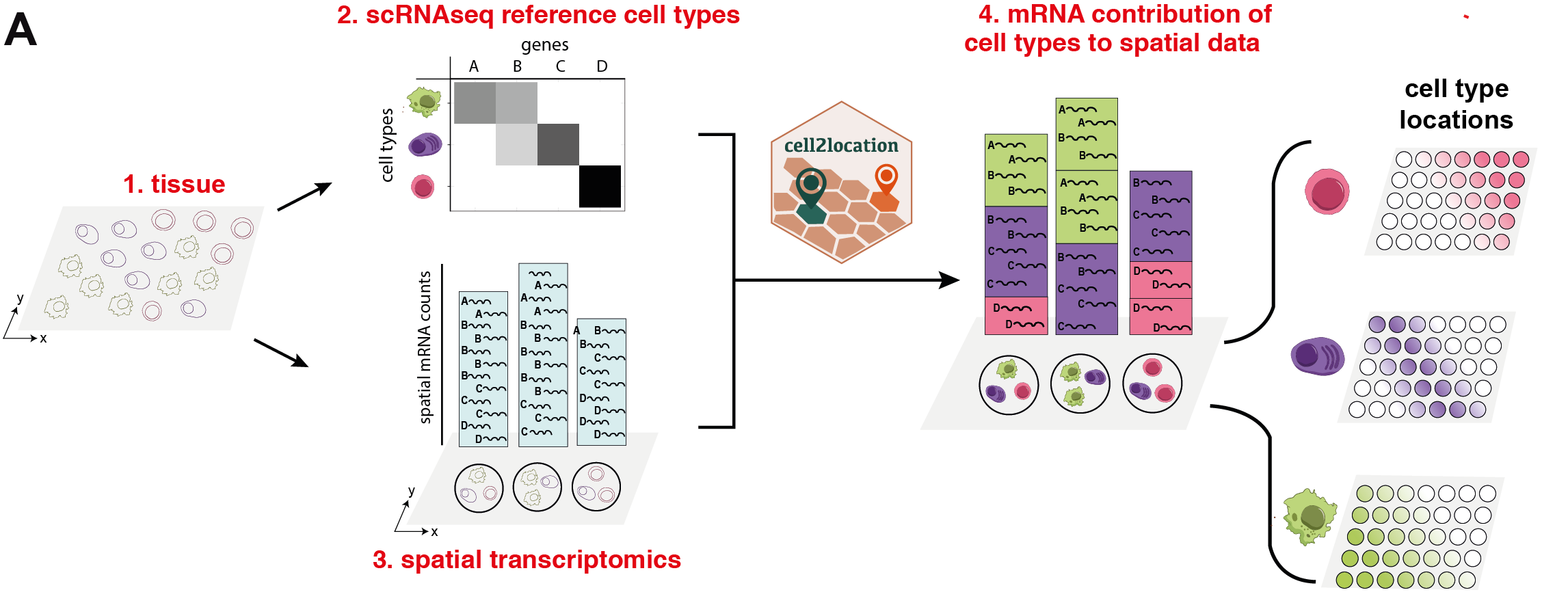
cell2location is a Bayesian model that integrates single-cell RNA-seq (scRNA-seq) and multi-cell spatial transcriptomics to map cell types at scale (Fig below). cell2location leverages reference signatures that are estimated from scRNA-seq profiles, for example using conventional clustering followed by estimation of average gene expression profiles. Based on these reference signatures, mRNA contributions from each of the defined cell types are estimated at each location in the spatial data, which gives rise to both cell type proportions as well as absolute densities of cell types in a spatially resolved manner. In this notebook, we examine and use estimated cell abundances of cell types to perform downstream analysis.

*Figure 1.* Overview of the spatial mapping approach and the workflow which are enabled by cell2location. From left to right: Single-cell RNA-seq and spatial transcriptomics profiles are generated from the same tissue (1). Cell2location takes reference cell type signatures derived from scRNA-seq and spatial transcriptomics data as input (2, 3). The model then decomposes spatially resolved multi-cell RNA counts matrices into the reference signatures, thereby establishing a spatial mapping of cell types (4).

Outline

The **cell2location** workflow consists of three sections:

1. Estimating reference expression signatures of cell types (1/3)

2. Spatially mapping cell types (2/3)

3. Results and downstream analysis (3/3, this notebook):

1. Loading cell2location model output

2. Visualisation of cell type locations

3. Automatic discrete region identification by clustering cell densities

4. Identify groups of co-located cell types using matrix factorisation (NMF)

Loading packages

import sys
import pickle
import scanpy as sc
import anndata
import numpy as np
import os

import cell2location

import matplotlib as mpl
from matplotlib import pyplot as plt

# scanpy prints a lot of warnings
import warnings
warnings.filterwarnings('ignore')

1. Loading cell2location model output

First, let’s load the cell2location results. In the export step of cell2location pipeline, cell type abundances across locations are added to sp_data as columns of sp_data.obs and all paramters of the model are exported to sp_data.uns['mod']. This anndata object and a csv file W.csv / W_q05.csv with cell locations are saved to the results directory.

Normally, you would have the output on your system (e.g. by running tutorial 2/3), however, you could also start with the output from our data portal:

results_folder = './results/mouse_brain_snrna/'
r = {'run_name': 'LocationModelLinearDependentWMultiExperiment_2experiments_59clusters_5563locations_12809genes'}

# defining useful function
def select_slide(adata, s, s_col='sample'):
    r""" Select data for one slide from the spatial anndata object.

    :param adata: Anndata object with multiple spatial samples
    :param s: name of selected sample
    :param s_col: column in adata.obs listing sample name for each location
    """

    slide = adata[adata.obs[s_col].isin([s]), :]
    s_keys = list(slide.uns['spatial'].keys())
    s_spatial = np.array(s_keys)[[s in k for k in s_keys]][0]

    slide.uns['spatial'] = {s_spatial: slide.uns['spatial'][s_spatial]}

    return slide

if os.path.exists(f'{results_folder}{r["run_name"]}') is not True:
    os.mkdir('./results')
    os.mkdir(f'{results_folder}')
    os.system(f'cd {results_folder} && wget https://cell2location.cog.sanger.ac.uk/tutorial/mouse_brain_visium_results/{["run_name"]}.zip')
    os.system(f'cd {results_folder} && unzip {r["run_name"]}.zip')

We load the results of the model saved into the adata_vis Anndata object:

sp_data_file = results_folder +r['run_name']+'/sp.h5ad'

adata_vis = anndata.read(sp_data_file)

2. Visualisation of cell type locations

First, we learn how to visualise cell type locations using the standard scanpy plotting tool sc.pl.spatial and our custom tool that visualises several cell types in one figure using colour interpolation cell2location.plt.mapping_video.plot_spatial.

Cell2location estimates the absolute cell and mRNA abundance of reference cells types. For both of these measures, 5% quantile of the posterior distribution are used to visualise the results, representing the confident level of cell abundance and mRNA count.

For completeness, for each visium section, sc.pl.spatial was used to produce 4 figure panels showing the locations of all cell types (cell and mRNA abundance, 5% and the mean of the posterior distribution), saved to r['run_name']/plots/spatial/.

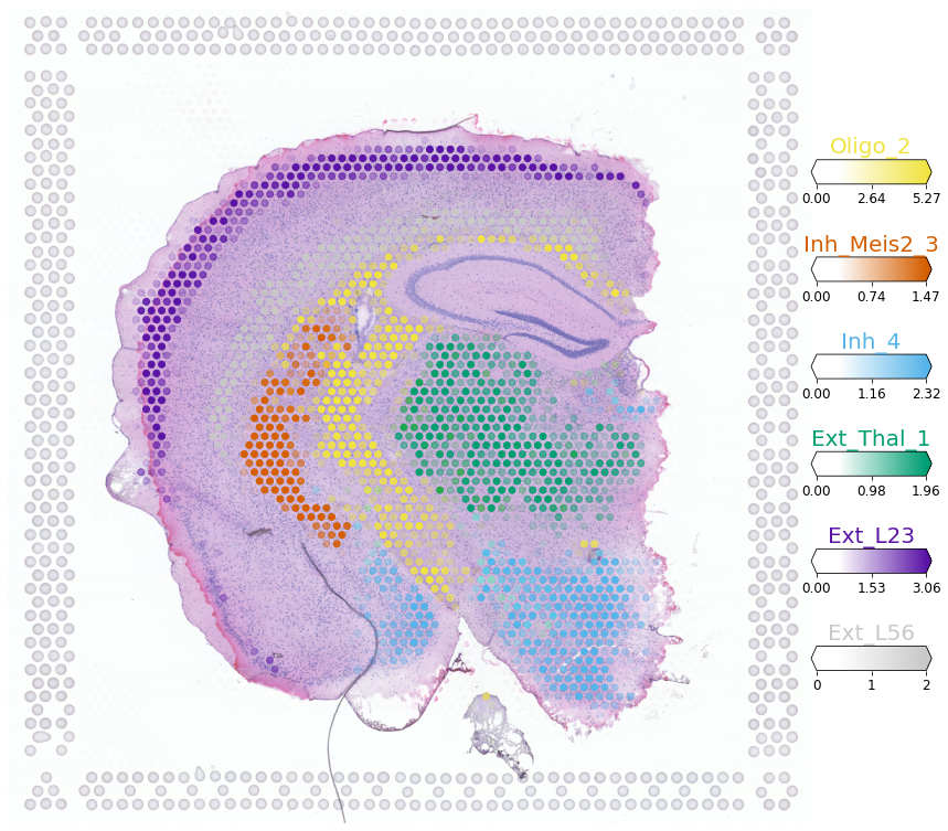
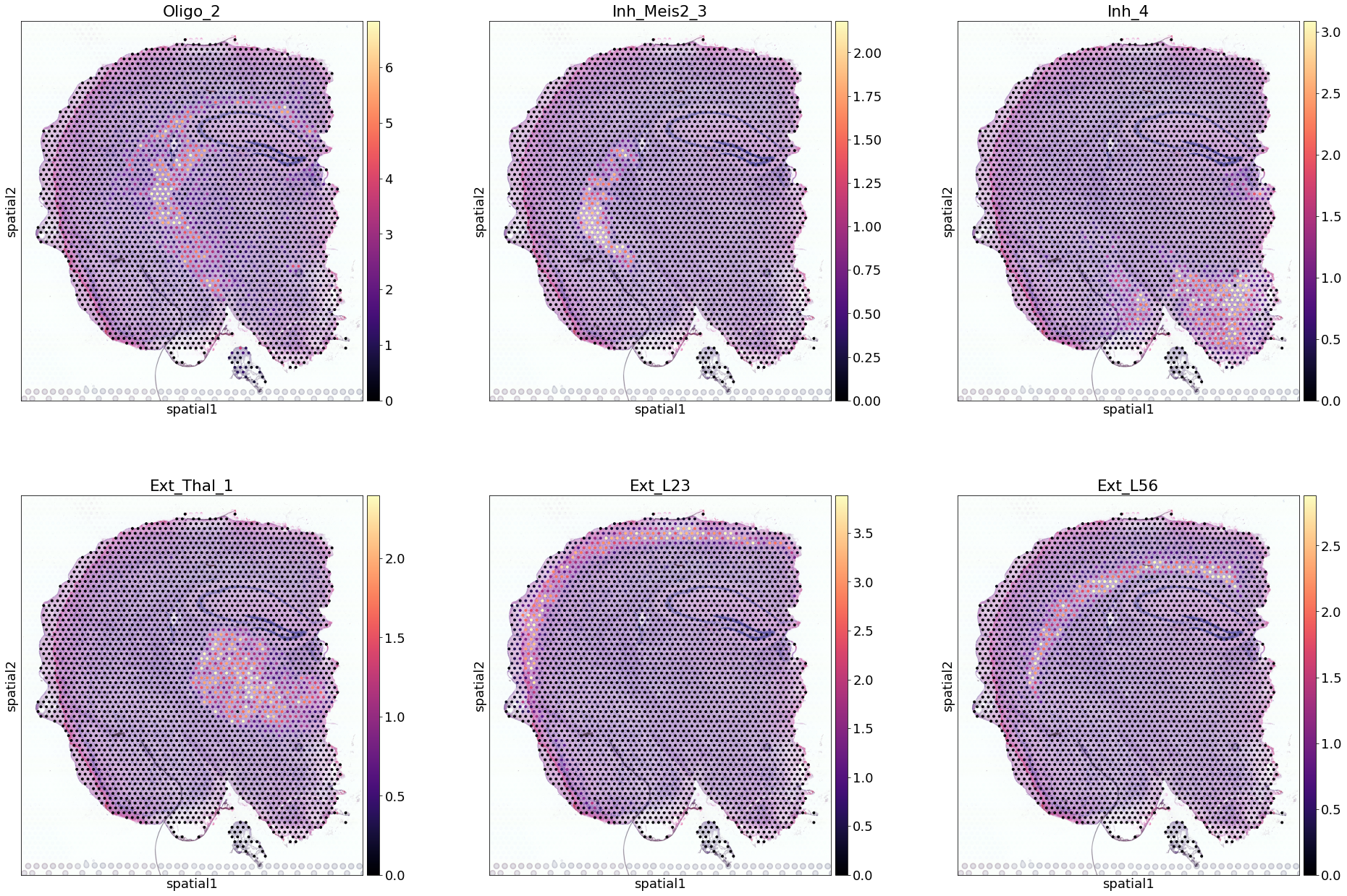
Here, we visualise locations of multiple cell types in one figure using absolute cell density (5% quantile), model parameter representing this is called q05_spot_factors. Six neuronal and glial cell types mapping to 6 distinct regions of the mouse brain are shown.

from cell2location.plt.mapping_video import plot_spatial

# select up to 6 clusters
sel_clust = ['Oligo_2', 'Inh_Meis2_3', 'Inh_4', 'Ext_Thal_1', 'Ext_L23', 'Ext_L56']
sel_clust_col = ['q05_spot_factors' + str(i) for i in sel_clust]

slide = select_slide(adata_vis, 'ST8059048')

with mpl.rc_context({'figure.figsize': (15, 15)}):
    fig = plot_spatial(slide.obs[sel_clust_col], labels=sel_clust,
                  coords=slide.obsm['spatial'] \
                          * list(slide.uns['spatial'].values())[0]['scalefactors']['tissue_hires_scalef'],
                  show_img=True, img_alpha=0.8,
                  style='fast', # fast or dark_background
                  img=list(slide.uns['spatial'].values())[0]['images']['hires'],
                  circle_diameter=6, colorbar_position='right')

Trying to set attribute `.uns` of view, copying.

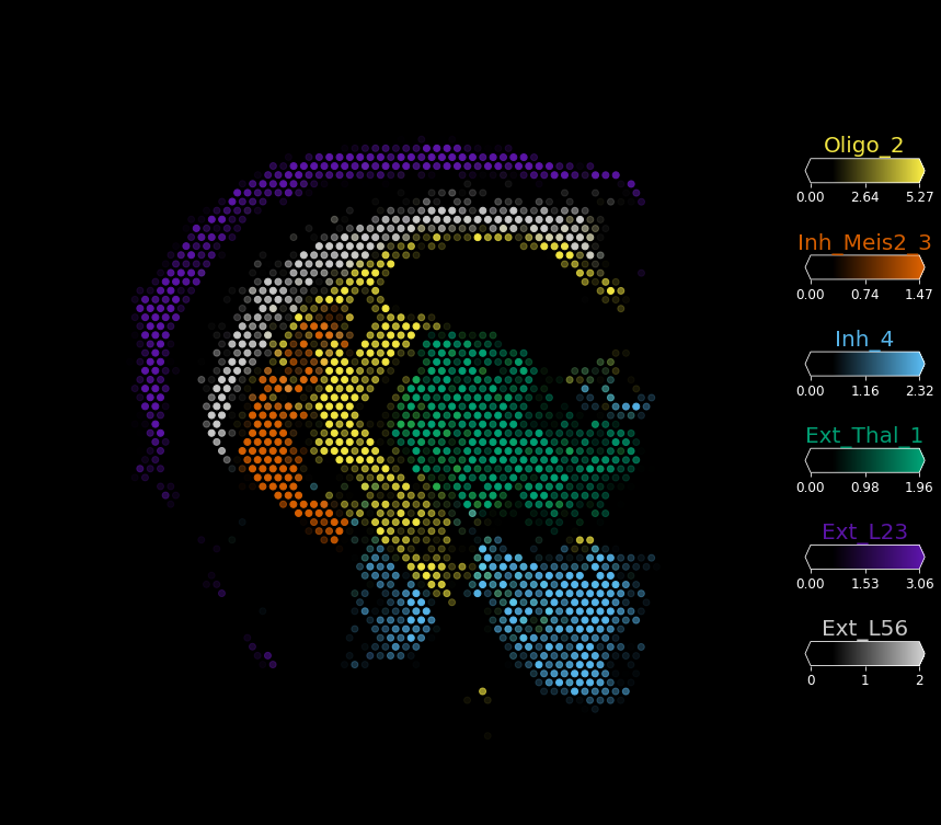
We can produce this visualisation in dark background by setting style='dark_background' and hiding the image img_alpha=0.

with mpl.rc_context({'figure.figsize': (15, 15)}):
    fig = plot_spatial(slide.obs[sel_clust_col], labels=sel_clust,
                  coords=slide.obsm['spatial'] \
                          * list(slide.uns['spatial'].values())[0]['scalefactors']['tissue_hires_scalef'],
                  show_img=True, img_alpha=0,
                  style='dark_background', # fast or dark_background
                  img=list(slide.uns['spatial'].values())[0]['images']['hires'],
                  circle_diameter=6, colorbar_position='right')

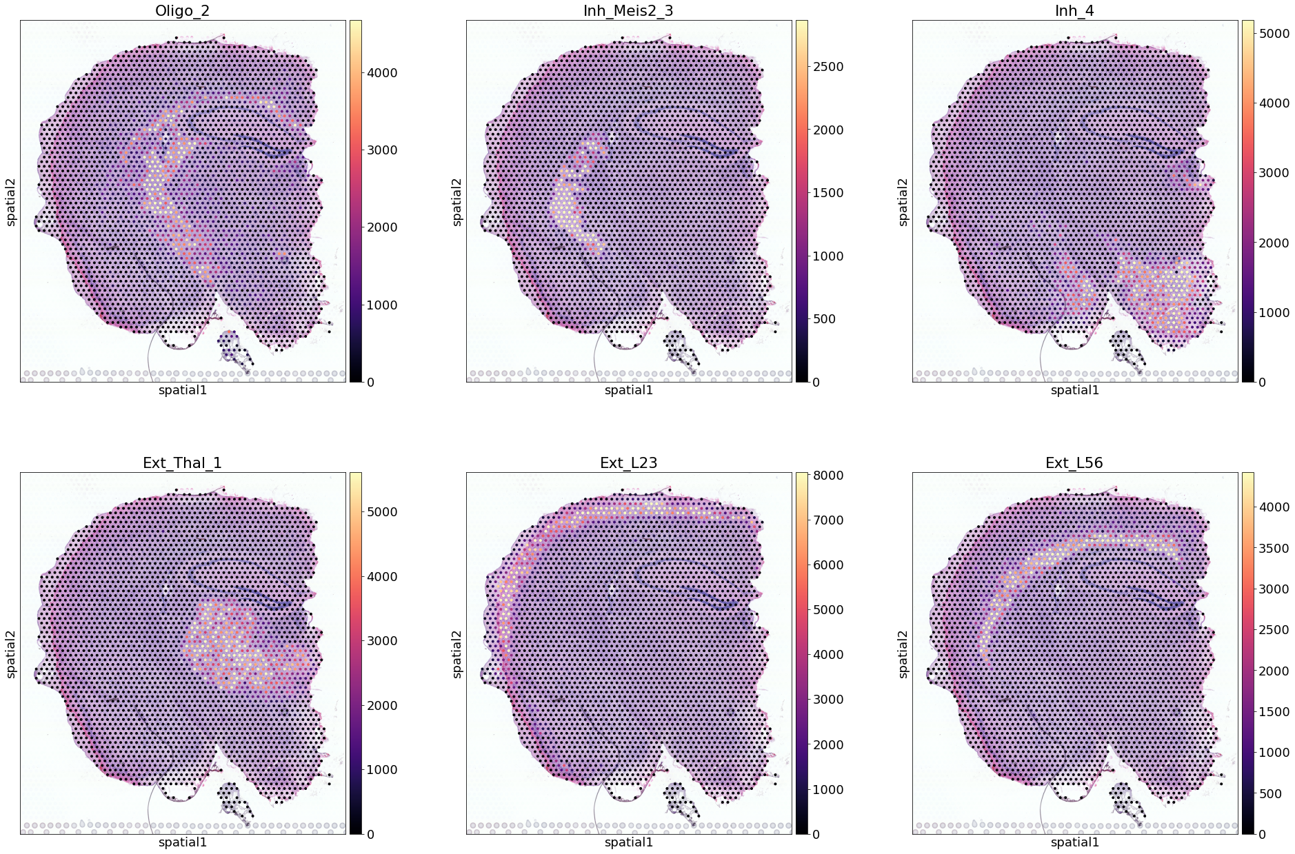
Now, we compare the cell abundance estimates (above) to the estimated mRNA abundance from each cell type. This is often useful for indentifying which cell types did not map to a particular tissue (see paper Fig S6, mRNA count < 50 - note max value on the color bars), model parameter representing this is called q05_nUMI_factors.

# select up to 6 clusters
sel_clust = ['Oligo_2', 'Inh_Meis2_3', 'Inh_4', 'Ext_Thal_1', 'Ext_L23', 'Ext_L56']
sel_clust_col = ['q05_nUMI_factors' + str(i) for i in sel_clust]

slide = select_slide(adata_vis, 'ST8059048')

with mpl.rc_context({'figure.figsize': (15, 15)}):
    fig = plot_spatial(slide.obs[sel_clust_col], labels=sel_clust,
                  coords=slide.obsm['spatial'] \
                          * list(slide.uns['spatial'].values())[0]['scalefactors']['tissue_hires_scalef'],
                  show_img=True, img_alpha=0.8, max_color_quantile=0.98,
                  img=list(slide.uns['spatial'].values())[0]['images']['hires'],
                  circle_diameter=6,  colorbar_position='right')

Trying to set attribute `.uns` of view, copying.

#sel_clust = ['Oligo_2', 'Inh_Meis2_3', 'Inh_4', 'Ext_Thal_1', 'Ext_L23', 'Ext_L56']
#sel_clust_col = ['q05_spot_factors' + str(i) for i in sel_clust]

# select one section correctly subsetting histology image data
slide = select_slide(adata_vis, 'ST8059048')

# plot with nice names
with mpl.rc_context({'figure.figsize': (10, 10), "font.size": 18}):
    # add slide.obs with nice names
    slide.obs[sel_clust] = (slide.obs[sel_clust_col])

    sc.pl.spatial(slide, cmap='magma',
                  color=sel_clust[0:6], # limit size in this notebook
                  ncols=3,
                  size=0.8, img_key='hires',
                  alpha_img=0.9,
                  vmin=0, vmax='p98'
                 )

Trying to set attribute `.uns` of view, copying.

Next, we show how to use the standard scanpy pipeline to plot cell locations over histology images (for more extensive information refer to scanpy):

sel_clust = ['Oligo_2', 'Inh_Meis2_3', 'Inh_4', 'Ext_Thal_1', 'Ext_L23', 'Ext_L56']
sel_clust_col = ['q05_spot_factors' + str(i) for i in sel_clust]

# select one section correctly subsetting histology image data
slide = select_slide(adata_vis, 'ST8059048')

# plot with nice names
with mpl.rc_context({'figure.figsize': (10, 10), "font.size": 18}):
    # add slide.obs with nice names
    slide.obs[sel_clust] = (slide.obs[sel_clust_col])

    sc.pl.spatial(slide, cmap='magma',
                  color=sel_clust[0:6], # limit size in this notebook
                  ncols=3,
                  size=0.8, img_key='hires',
                  alpha_img=0.9,
                  vmin=0, vmax='p99.2'
                 )

Trying to set attribute `.uns` of view, copying.

3. Identifying tissue regions by clustering

We identify tissue regions that differ in their cell composition by clustering locations using cell abundance estimated by cell2location.

We find tissue regions by clustering Visium spots using estimated cell abundance each cell type. We constuct a K-nearest neigbour (KNN) graph representing similarity of locations in estimated cell abundance and then apply Leiden clustering. The number of KNN neighbours should be adapted to size of dataset and the size of anatomically defined regions (e.i. hippocampus regions are rather small so could be masked by large n_neighbors). This can be done for a range KNN neighbours and Leiden clustering resolutions until a clustering matching the anatomical structure of the tissue is obtained.

The clustering is done jointly across all Visium sections / batches, hence the region identities are directly comparable. When there are strong technical effects between multiple batches (not the case here) sc.external.pp.bbknn can be used to account for those effects during the KNN construction.

The resulting clusters are saved in adata_vis.obs['region_cluster'].

sample_type = 'q05_nUMI_factors'
col_ind = [sample_type in i for i in adata_vis.obs.columns.tolist()]
adata_vis.obsm[sample_type] = adata_vis.obs.loc[:,col_ind].values

# compute KNN using the cell2location output
sc.pp.neighbors(adata_vis, use_rep=sample_type,
                n_neighbors = 20)

# Cluster spots into regions using scanpy
sc.tl.leiden(adata_vis, resolution=1)

# add region as categorical variable
adata_vis.obs["region_cluster"] = adata_vis.obs["leiden"]
adata_vis.obs["region_cluster"] =  adata_vis.obs["region_cluster"].astype("category")

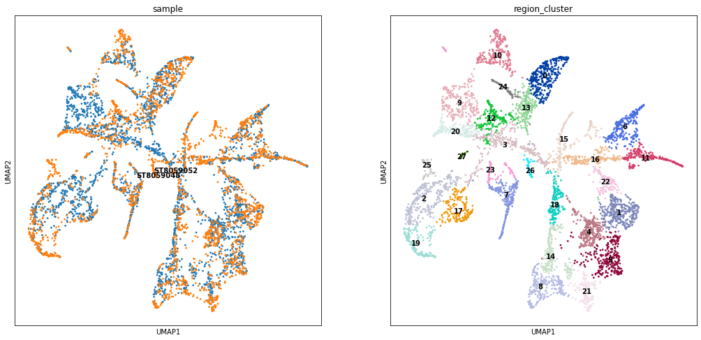
Visualise the regions in UMAP based on cell abundances and in 2D

Here we use the same KNN graph representing similarity locations in terms of cell abundance to perform UMAP projection of all locations. We can see that cell2location successfully integrated the 2 sections. You can see that the regions with analogous position in the cortex (2D below) are composed out of spots coming from both samples (e.g. region cluster 14, 16, 0 - cortical layers L4, L5 and L6).

sc.tl.umap(adata_vis, min_dist = 0.3, spread = 1)

with mpl.rc_context({'figure.figsize': (8, 8)}):
    sc.pl.umap(adata_vis, color=['sample', 'region_cluster'], size=30,
               color_map = 'RdPu', ncols = 2, legend_loc='on data',
               legend_fontsize=10)

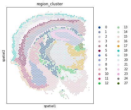
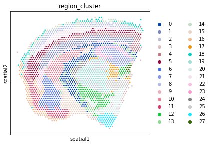
# Plot the region identity of each location in 2D space
# Plotting UMAP of integrated datasets before 2D plots of separate sections ensures
# consistency of colour scheme via `adata_vis.uns['region_cluster_colors']`.
with mpl.rc_context({'figure.figsize': (5, 6)}):
    sc.pl.spatial(select_slide(adata_vis, 'ST8059048'),
                  color=["region_cluster"], img_key=None
                );
    sc.pl.spatial(select_slide(adata_vis, 'ST8059052'),
                  color=["region_cluster"], img_key=None
                )

Trying to set attribute `.uns` of view, copying.

Trying to set attribute `.uns` of view, copying.

Export regions for import to 10X Loupe Browser

Our region maps can be visualised over the histology image and explored interactively using the 10X Loupe Browser (please refer to 10X website for instructions).

# save maps for each sample separately
sam = np.array(adata_vis.obs['sample'])
for i in np.unique(sam):

    s1 = adata_vis.obs[['region_cluster']]
    s1 = s1.loc[sam == i]
    s1.index = [x[10:] for x in s1.index]
    s1.index.name = 'Barcode'

    s1.to_csv(results_folder +r['run_name']+'/region_cluster29_' + i + '.csv')

4. Identify groups of co-located cell types using matrix factorisation

Here, we use estimated cell abundances as an input to non-negative matrix factorisation to identify groups of co-located cell types \(R\), which can be interpreted as cellular compartments or tissue zones. See paper section 4 and Supplemenary Methods for details. Intuitively, we hypothesise that cell interactions can drive linear dependencies in cell type abundance, which can be estimated via NMF Supplemenary Methods section 4.2. In addition, we observed that tissues with a high degree of spatial interlacing of cellular comparments such as the human lymph nodes are better described by NMF that by discrete clustering (see paper Fig S16)

Tip If you want to find a few most disctinct cellular compartments, use a small number of factors. If you want to find very strong co-location signal and assume that most cell types don’t co-locate, use a lot of factors (> 30 - used here). In practice, it is better to train NMF for a range of factors \(R={5, .., 30}\) and select \(R\) as a balance between capturing fine tissue zones and splitting known compartments

Below we show how to perform this analysis. First, we initialise this model and train it several times to evaluate consitency of identified compartments.

# number of cell type combinations - educated guess assuming that most cell types don't co-locate
n_fact = int(30)

# extract cell abundance from cell2location
X_data = adata_vis.uns['mod']['post_sample_q05']['spot_factors']

import cell2location.models as c2l
# create model class
mod_sk = c2l.CoLocatedGroupsSklearnNMF(n_fact, X_data,
        n_iter = 10000,
        verbose = True,
        var_names=adata_vis.uns['mod']['fact_names'],
        obs_names=adata_vis.obs_names,
        fact_names=['fact_' + str(i) for i in range(n_fact)],
        sample_id=adata_vis.obs['sample'],
        init='random', random_state=0,
        nmf_kwd_args={'tol':0.0001})

# train 5 times to evaluate stability
mod_sk.fit(n=5, n_type='restart')

init_1 - iterations until convergence: 1119
init_2 - iterations until convergence: 1214
init_3 - iterations until convergence: 1137
init_4 - iterations until convergence: 1133
init_5 - iterations until convergence: 1085

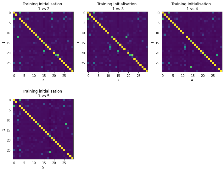
Now, let’s examine a few diagnostic plots. First, you can see that most cell type combinations are consistent between training restarts of this model (diagonal with high correlation). The first restart is used (y-axis) so we can take a note that factors 21, 23, 25 (0-based) is not very robust.

## Do some diagnostics
# evaluate stability by comparing trainin restarts

with mpl.rc_context({'figure.figsize': (10, 8)}):
    mod_sk.evaluate_stability('cell_type_factors', align=True)

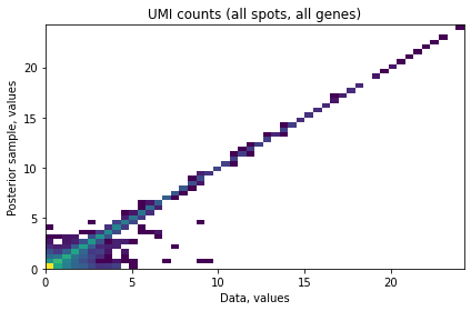
Next we evaluate the accuracy of NMF the cell type groups at explaining the abundace of individual cell types. You should see a diagonal 2D histogram comparing the input cell density data (X-axis) and imputed values from the model (Y-axis). Here we a few minor deviations for low abundance cell types.

# evaluate accuracy of the model
mod_sk.compute_expected()
mod_sk.plot_posterior_mu_vs_data()

Finally, let’s investigate the composition of each NMF cell type group. We use our model to compute the relative contribution of NMF groups to each cell type ('cell_type_fractions' e.g. 45% of cell abundance of Astro_THAL_hab can be explained by fact_10). Note: factors are exchangeable so while you find consistent factors, each model training restart will output those factors in a different order.

Here we export these parameters from the model into adata_vis.uns['mod_sklearn'] in the spatial anndata object, and print the cell types most specific to each NMF group:

# extract parameters into DataFrames
mod_sk.sample2df(node_name='nUMI_factors', ct_node_name = 'cell_type_factors')

# export results to scanpy object
adata_vis = mod_sk.annotate_adata(adata_vis) # as columns to .obs
adata_vis = mod_sk.export2adata(adata_vis, slot_name='mod_sklearn') # as a slot in .uns

# print the fraction of cells of each type located to each combination
mod_sk.print_gene_loadings(loadings_attr='cell_type_fractions',
                         gene_fact_name='cell_type_fractions')

	top-1	top-2	top-3	top-4	top-5	top-6	top-7	top-8	top-9	top-10
mean_cell_type_factorsfact_0	Ext_Hpc_DG2: 0.88	Nb_1: 0.26	Astro_HPC: 0.16	Inh_Lamp5: 0.096	Ext_Unk_1: 0.082	Ext_Hpc_DG1: 0.061	Inh_Vip: 0.055	Astro_STR: 0.043	Astro_AMY_CTX: 0.042	Nb_2: 0.023
mean_cell_type_factorsfact_1	Ext_Hpc_CA3: 0.99	Ext_Hpc_CA2: 0.35	Unk_1: 0.23	Astro_STR: 0.053	Unk_2: 0.039	Nb_1: 0.033	Astro_HPC: 0.027	Endo: 0.013	Inh_5: 0.01	Astro_AMY: 0.0071
mean_cell_type_factorsfact_2	Oligo_1: 0.91	OPC_2: 0.56	Astro_STR: 0.046	Astro_WM: 0.044	Micro: 0.043	Endo: 0.033	Astro_THAL_hab: 0.016	Oligo_2: 0.013	Inh_Sst: 0.012	Inh_Vip: 0.012
mean_cell_type_factorsfact_3	Ext_Hpc_CA1: 0.99	Ext_Hpc_CA2: 0.18	Astro_HPC: 0.061	Unk_1: 0.049	Astro_STR: 0.036	Inh_Lamp5: 0.019	Micro: 0.019	Nb_2: 0.013	Inh_Vip: 0.012	Nb_1: 0.01
mean_cell_type_factorsfact_4	Ext_Pir: 0.98	Astro_AMY_CTX: 0.1	Ext_Unk_1: 0.04	Unk_1: 0.021	Micro: 0.021	Inh_Lamp5: 0.019	OPC_1: 0.017	Inh_Meis2_1: 0.013	Unk_2: 0.0083	Inh_Vip: 0.0074
mean_cell_type_factorsfact_5	Ext_ClauPyr: 0.99	Inh_Lamp5: 0.027	Ext_L56: 0.022	Inh_Sst: 0.02	Astro_AMY_CTX: 0.019	OPC_1: 0.018	OPC_2: 0.016	Astro_CTX: 0.011	Ext_L6: 0.0098	Nb_2: 0.0055
mean_cell_type_factorsfact_6	Ext_Amy_2: 0.99	Astro_AMY_CTX: 0.27	Astro_AMY: 0.25	Inh_Vip: 0.2	Inh_Sst: 0.15	Unk_1: 0.12	Inh_Meis2_1: 0.12	OPC_1: 0.1	Ext_L5_3: 0.065	Micro: 0.06
mean_cell_type_factorsfact_7	LowQ_1: 0.99	Endo: 0.047	Inh_5: 0.039	Astro_WM: 0.023	Micro: 0.018	Astro_THAL_hab: 0.0031	Inh_1: 0.0018	Unk_2: 0.00075	Ext_L5_3: 0.00061	Astro_HYPO: 0.00048
mean_cell_type_factorsfact_8	Ext_L25: 0.9	Astro_CTX: 0.14	Ext_Med: 0.12	Inh_Pvalb: 0.058	Endo: 0.03	Micro: 0.028	Inh_Vip: 0.026	Ext_L23: 0.015	Ext_L5_1: 0.012	Ext_L56: 0.01
mean_cell_type_factorsfact_9	Ext_L56: 0.85	Ext_L6: 0.63	Astro_STR: 0.073	Micro: 0.029	OPC_1: 0.026	OPC_2: 0.016	Inh_Pvalb: 0.013	Astro_CTX: 0.011	Inh_Lamp5: 0.01	LowQ_2: 0.0076
mean_cell_type_factorsfact_10	Ext_L5_2: 0.98	LowQ_2: 0.59	Inh_5: 0.48	Ext_Med: 0.24	Inh_Pvalb: 0.086	Ext_L56: 0.057	Astro_CTX: 0.04	Unk_1: 0.017	Ext_L5_1: 0.016	Inh_2: 0.016
mean_cell_type_factorsfact_11	Inh_4: 0.94	Inh_3: 0.82	Unk_2: 0.44	Astro_HYPO: 0.44	OPC_1: 0.14	Astro_THAL_hab: 0.083	Inh_1: 0.072	Endo: 0.055	Inh_2: 0.052	Nb_1: 0.038
mean_cell_type_factorsfact_12	Inh_Meis2_3: 0.97	Inh_Meis2_1: 0.17	Astro_AMY: 0.17	Astro_AMY_CTX: 0.14	Astro_HPC: 0.13	Astro_STR: 0.065	OPC_1: 0.058	Micro: 0.055	Endo: 0.025	Inh_Meis2_2: 0.02
mean_cell_type_factorsfact_13	Astro_CTX: 0.71	Ext_Med: 0.51	Inh_Lamp5: 0.37	Endo: 0.32	Astro_HPC: 0.28	LowQ_2: 0.21	Micro: 0.18	Astro_STR: 0.14	Inh_Pvalb: 0.097	Ext_L25: 0.074
mean_cell_type_factorsfact_14	Ext_Hpc_DG1: 0.94	Nb_1: 0.23	Nb_2: 0.14	Ext_Hpc_DG2: 0.12	Ext_Hpc_CA2: 0.032	Unk_2: 0.015	Micro: 0.0026	Ext_Amy_2: 0.001	Unk_1: 0.00069	Inh_1: 0.00041
mean_cell_type_factorsfact_15	Ext_Thal_1: 1.0	Astro_THAL_lat: 0.5	Astro_THAL_med: 0.33	Inh_Meis2_4: 0.058	Endo: 0.035	OPC_1: 0.033	Oligo_1: 0.026	Inh_5: 0.024	Micro: 0.021	Oligo_2: 0.011
mean_cell_type_factorsfact_16	Unk_1: 0.5	Ext_Hpc_CA2: 0.28	Inh_Sst: 0.25	Ext_L6: 0.23	Astro_AMY_CTX: 0.22	Inh_Vip: 0.13	Ext_L5_3: 0.13	Unk_2: 0.12	Inh_Lamp5: 0.089	Astro_HPC: 0.087
mean_cell_type_factorsfact_17	Ext_Thal_2: 0.99	Astro_THAL_med: 0.35	Astro_HYPO: 0.086	Astro_THAL_lat: 0.065	Unk_2: 0.063	Astro_THAL_hab: 0.052	OPC_1: 0.033	Micro: 0.017	Oligo_1: 0.013	Endo: 0.0078
mean_cell_type_factorsfact_18	Inh_1: 0.91	Inh_Meis2_1: 0.61	Ext_Unk_1: 0.18	Astro_AMY: 0.1	Inh_4: 0.058	OPC_1: 0.055	Astro_HYPO: 0.042	Astro_AMY_CTX: 0.04	Ext_L5_3: 0.04	Astro_THAL_hab: 0.012
mean_cell_type_factorsfact_19	Ext_Unk_2: 0.99	Inh_2: 0.89	Inh_5: 0.35	Astro_THAL_lat: 0.33	Astro_HYPO: 0.26	Inh_Meis2_4: 0.22	Astro_THAL_med: 0.15	Endo: 0.058	OPC_1: 0.015	Oligo_2: 0.015
mean_cell_type_factorsfact_20	Ext_L6B: 0.99	Ext_L5_3: 0.76	Astro_STR: 0.16	Inh_Sst: 0.058	Inh_Lamp5: 0.054	Endo: 0.052	Inh_Vip: 0.049	Micro: 0.04	Inh_Meis2_1: 0.02	Astro_HPC: 0.013
mean_cell_type_factorsfact_21	Ext_Amy_1: 0.99	Ext_Unk_1: 0.39	Astro_AMY: 0.35	Inh_Sst: 0.15	Inh_Vip: 0.13	Inh_Lamp5: 0.083	OPC_1: 0.061	Nb_1: 0.06	Astro_AMY_CTX: 0.049	Nb_2: 0.036
mean_cell_type_factorsfact_22	Ext_L23: 0.94	Inh_Vip: 0.17	Inh_Lamp5: 0.11	Astro_AMY_CTX: 0.074	OPC_1: 0.071	Micro: 0.066	Ext_Med: 0.065	Astro_CTX: 0.024	Endo: 0.017	Ext_Unk_1: 0.015
mean_cell_type_factorsfact_23	Oligo_2: 0.92	Astro_THAL_hab: 0.23	OPC_2: 0.14	Micro: 0.12	OPC_1: 0.1	Inh_Meis2_4: 0.087	Astro_WM: 0.083	Endo: 0.049	Astro_STR: 0.035	Oligo_1: 0.031
mean_cell_type_factorsfact_24	Inh_Pvalb: 0.73	Inh_Meis2_4: 0.64	Ext_Hpc_CA2: 0.16	Inh_Sst: 0.12	Inh_Vip: 0.096	LowQ_2: 0.072	Ext_Med: 0.059	Nb_1: 0.057	Inh_5: 0.056	Astro_THAL_lat: 0.039
mean_cell_type_factorsfact_25	Ext_Unk_3: 1.0	Inh_3: 0.16	Astro_THAL_med: 0.14	Astro_HYPO: 0.11	Astro_THAL_hab: 0.071	Endo: 0.033	OPC_1: 0.029	Astro_THAL_lat: 0.027	Unk_2: 0.0039	Inh_5: 0.0039
mean_cell_type_factorsfact_26	Inh_Meis2_2: 0.98	Astro_STR: 0.17	Astro_HPC: 0.059	Inh_Meis2_3: 0.026	Inh_Sst: 0.016	Oligo_2: 0.0092	Astro_CTX: 0.0085	Oligo_1: 0.0058	Micro: 0.0042	Unk_2: 0.0035
mean_cell_type_factorsfact_27	Ext_L5_1: 0.94	Inh_Sst: 0.14	Ext_L6: 0.099	LowQ_2: 0.096	Astro_CTX: 0.037	Micro: 0.034	Inh_Vip: 0.024	OPC_2: 0.023	OPC_1: 0.017	Ext_L5_2: 0.016
mean_cell_type_factorsfact_28	Astro_WM: 0.83	Nb_2: 0.66	Ext_Unk_1: 0.22	Nb_1: 0.19	OPC_2: 0.18	Unk_2: 0.17	Astro_HPC: 0.15	Micro: 0.14	Endo: 0.091	Astro_STR: 0.074
mean_cell_type_factorsfact_29	Inh_6: 1.0	Astro_THAL_hab: 0.45	Unk_2: 0.054	Endo: 0.023	OPC_2: 0.022	Astro_WM: 0.019	Inh_2: 0.013	OPC_1: 0.013	Astro_HYPO: 0.011	Inh_5: 0.0066

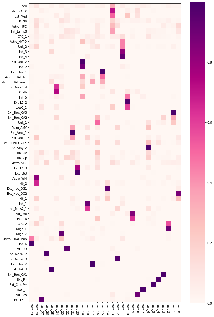
A convenient way to explore which cell types show co-location signals is by using a heatmap. Here, we note that most factors correspond to a single neuron type (e.g. Ext_Pir), however, many neurone types are associated with corresponding regional astrocyte subtypes, such as

1. fact_10 - Astro_THAL_hab and Inh_6 neurones

2. fact_21 - Astro_AMY and Ext_Amy_1 neurones

3. fact_14 - Astro_HPC and Ext_Hpc_DG2 neurones

# make nice names
from re import sub
mod_sk.cell_type_fractions.columns = [sub('mean_cell_type_factors', '', i)
                                      for i in mod_sk.cell_type_fractions.columns]

# plot co-occuring cell type combinations
mod_sk.plot_gene_loadings(mod_sk.var_names_read, mod_sk.var_names_read,
                        fact_filt=mod_sk.fact_filt,
                        loadings_attr='cell_type_fractions',
                        gene_fact_name='cell_type_fractions',
                        cmap='RdPu', figsize=[10, 15])

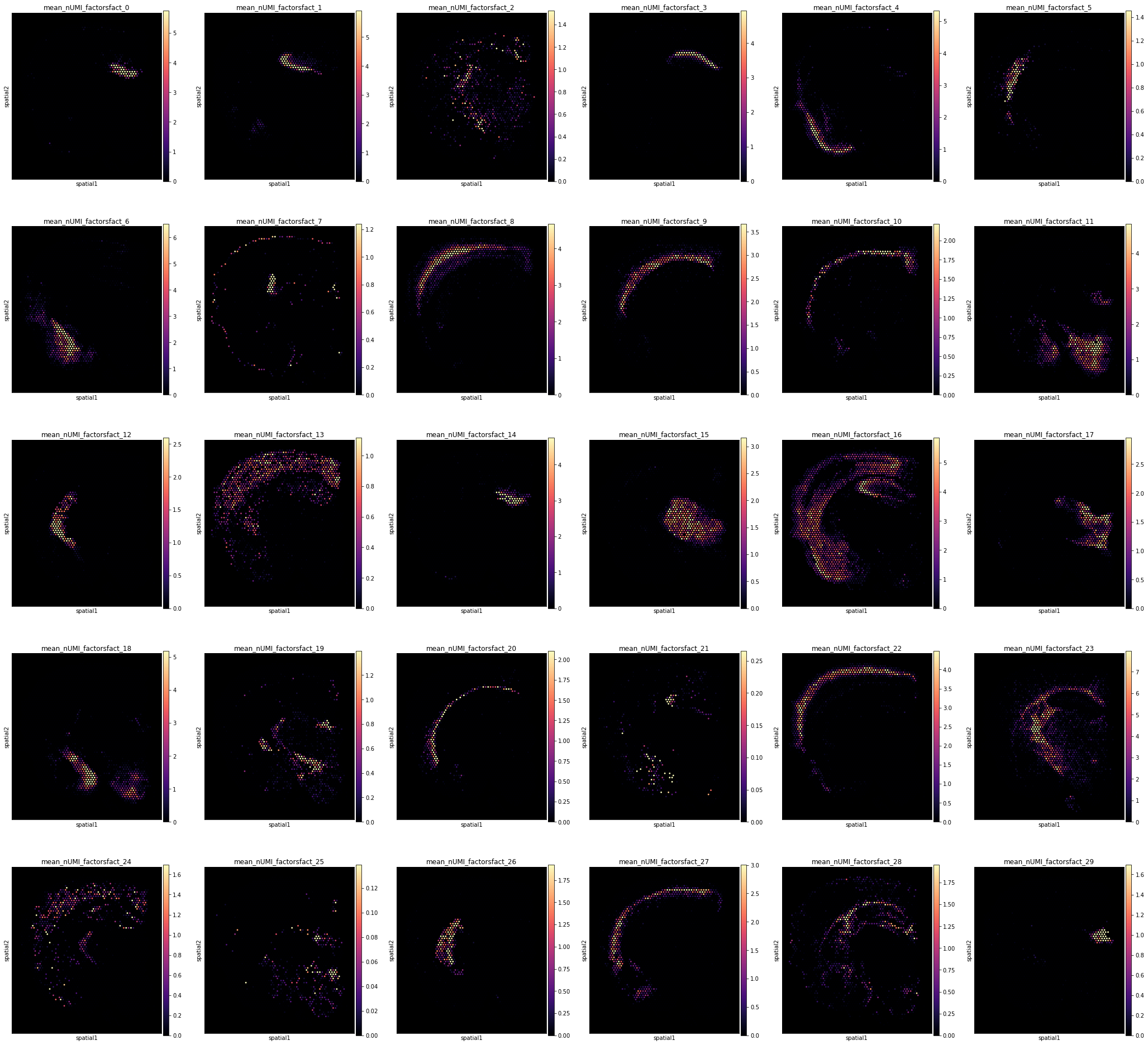
Finally, we need to examine the abundance of each cell type group across locations:

# plot cell density in each combination
with mpl.rc_context({'figure.figsize': (5, 6), 'axes.facecolor': 'black'}):

    # select one section correctly subsetting histology image data
    slide = select_slide(adata_vis, 'ST8059048')

    sc.pl.spatial(slide,
                  cmap='magma',
                  color=mod_sk.location_factors_df.columns,
                  ncols=6,
                  size=1, img_key='hires',
                  alpha_img=0,
                  vmin=0, vmax='p99.2'
                 )

Trying to set attribute `.uns` of view, copying.

Now we save the NMF model object to work with later (rememeber, every time you train the model, factors with the same composition will have a different order):

# save co-location models object
def pickle_model(mod, path, file_suffix=''):
    file = path + 'model_' + str(mod.__class__.__name__) + '_' + str(mod.n_fact) + '_' + file_suffix + ".p"
    pickle.dump({'mod': mod, 'fact_names': mod.fact_names}, file = open(file, "wb"))
    print(file)

pickle_model(mod_sk, results_folder +r['run_name'] + '/', file_suffix='')

./results/mouse_brain_snrna/LocationModelLinearDependentWMultiExperiment_2experiments_59clusters_5563locations_12809genes/model_CoLocatedGroupsSklearnNMF_30_.p

It is often useful to train NMF for a range of factors \(R\) to select most meaningful cell type groups

To aid this analysis, we wrapped the analysis shown above into a pipeline that automates training the NMF model with varying number of factors (including export of the same plots and data as shown above).

from cell2location import run_colocation
res_dict, adata_vis = run_colocation(
                   adata_vis, model_name='CoLocatedGroupsSklearnNMF',
                   verbose=False, return_all=True,

                   train_args={
                    'n_fact': np.arange(10, 40), # IMPORTANT: range of number of factors (10-40 here)
                    'n_iter': 20000, # maximum number of training iterations

                    'sample_name_col': 'sample', # columns in adata_vis.obs that identifies sample

                    'mode': 'normal',
                    'n_type': 'restart', 'n_restarts': 5 # number of training restarts
                   },

                   model_kwargs={'init': 'random', 'random_state': 0, 'nmf_kwd_args': {'tol': 0.00001}},

                   posterior_args={},
                   export_args={'path': results_folder + 'std_model/'+r['run_name']+'/CoLocatedComb/',
                                'run_name_suffix': ''})

Export results

Save resulting anndata object that now include region clustering and co-located cell type groups.

adata_file = results_folder +r['run_name']+'/sp_with_clusters.h5ad'
adata_vis.write(adata_file)
adata_file

'./results/mouse_brain_snrna/LocationModelLinearDependentWMultiExperiment_2experiments_59clusters_5563locations_12809genes/sp_with_clusters.h5ad'

Modules and their versions used for this analysis

import sys
for module in sys.modules:
    try:
        print(module,sys.modules[module].__version__)
    except:
        try:
            if  type(sys.modules[module].version) is str:
                print(module,sys.modules[module].version)
            else:
                print(module,sys.modules[module].version())
        except:
            try:
                print(module,sys.modules[module].VERSION)
            except:
                pass

sys 3.7.10 | packaged by conda-forge | (default, Feb 19 2021, 16:07:37)
[GCC 9.3.0]
ipykernel 6.2.0
ipykernel._version 6.2.0
json 2.0.9
re 2.2.1
ipython_genutils 0.2.0
ipython_genutils._version 0.2.0
zlib 1.0
platform 1.0.8
jupyter_client 6.1.12
jupyter_client._version 6.1.12
zmq 22.2.1
ctypes 1.1.0
_ctypes 1.1.0
zmq.backend.cython 40304
zmq.backend.cython.constants 40304
zmq.sugar 22.2.1
zmq.sugar.constants 40304
zmq.sugar.version 22.2.1
traitlets 5.0.5
traitlets._version 5.0.5
logging 0.5.1.2
argparse 1.1
jupyter_core 4.7.1
jupyter_core.version 4.7.1
tornado 6.1
colorama 0.4.4
_curses b'2.2'
IPython 7.26.0
IPython.core.release 7.26.0
IPython.core.crashhandler 7.26.0
pygments 2.10.0
pexpect 4.8.0
ptyprocess 0.7.0
decorator 5.0.9
pickleshare 0.7.5
backcall 0.2.0
sqlite3 2.6.0
sqlite3.dbapi2 2.6.0
_sqlite3 2.6.0
prompt_toolkit 3.0.19
wcwidth 0.2.5
jedi 0.18.0
parso 0.8.2
IPython.core.magics.code 7.26.0
urllib.request 3.7
dateutil 2.8.2
dateutil._version 2.8.2
six 1.16.0
decimal 1.70
_decimal 1.70
distutils 3.7.10
scanpy 1.8.1
scanpy._metadata 1.8.1
packaging 21.0
packaging.__about__ 21.0
importlib_metadata 1.7.0
csv 1.0
_csv 1.0
numpy 1.21.2
numpy.core 1.21.2
numpy.version 1.21.2
numpy.core._multiarray_umath 3.1
numpy.lib 1.21.2
numpy.linalg._umath_linalg 0.1.5
scipy 1.7.1
scipy.version 1.7.1
anndata 0.7.6
anndata._metadata 0.7.6
h5py 3.3.0
h5py.version 3.3.0
cached_property 1.5.2
natsort 7.1.1
pandas 1.3.2
pytz 2021.1
numexpr 2.7.3
numexpr.version 2.7.3
sinfo 0.3.1
stdlib_list v0.7.0
numba 0.53.1
yaml 5.4.1
llvmlite 0.36.0
pkg_resources._vendor.appdirs 1.4.3
pkg_resources.extern.appdirs 1.4.3
pkg_resources._vendor.packaging 20.4
pkg_resources._vendor.packaging.__about__ 20.4
pkg_resources.extern.packaging 20.4
pkg_resources._vendor.pyparsing 2.2.1
pkg_resources.extern.pyparsing 2.2.1
numba.misc.appdirs 1.4.1
sklearn 0.24.2
sklearn.base 0.24.2
joblib 1.0.1
joblib.externals.loky 2.9.0
joblib.externals.cloudpickle 1.6.0
scipy._lib.decorator 4.0.5
scipy.linalg._fblas b'$Revision: $'
scipy.linalg._flapack b'$Revision: $'
scipy.linalg._flinalg b'$Revision: $'
scipy.special.specfun b'$Revision: $'
scipy.ndimage 2.0
scipy.optimize.minpack2 b'$Revision: $'
scipy.sparse.linalg.isolve._iterative b'$Revision: $'
scipy.sparse.linalg.eigen.arpack._arpack b'$Revision: $'
scipy.optimize._lbfgsb b'$Revision: $'
scipy.optimize._cobyla b'$Revision: $'
scipy.optimize._slsqp b'$Revision: $'
scipy.optimize._minpack  1.10
scipy.optimize.__nnls b'$Revision: $'
scipy.linalg._interpolative b'$Revision: $'
scipy.integrate._odepack  1.9
scipy.integrate._quadpack  1.13
scipy.integrate._ode $Id$
scipy.integrate.vode b'$Revision: $'
scipy.integrate._dop b'$Revision: $'
scipy.integrate.lsoda b'$Revision: $'
scipy.interpolate._fitpack  1.7
scipy.interpolate.dfitpack b'$Revision: $'
scipy.stats.statlib b'$Revision: $'
scipy.stats.mvn b'$Revision: $'
sklearn.utils._joblib 1.0.1
leidenalg 0.8.7
igraph 0.9.6
texttable 1.6.4
igraph.version 0.9.6
leidenalg.version 0.8.7
louvain 0.7.0
matplotlib 3.4.3
PIL 8.3.1
PIL._version 8.3.1
PIL.Image 8.3.1
defusedxml 0.7.1
xml.etree.ElementTree 1.3.0
cffi 1.14.6
pyparsing 2.4.7
cycler 0.10.0
kiwisolver 1.3.1
tables 3.6.1
umap 0.5.1
_cffi_backend 1.14.6
pycparser 2.20
pycparser.ply 3.9
pycparser.ply.yacc 3.10
pycparser.ply.lex 3.10
pynndescent 0.5.4
theano 1.0.5
theano.version 1.0.5
mkl 2.4.0
scipy._lib._uarray 0.5.1+49.g4c3f1d7.scipy
scipy.signal.spline 0.2
plotnine 0.7.0
patsy 0.5.1
patsy.version 0.5.1
mizani 0.7.3
palettable 3.3.0
mizani.external.husl 4.0.3
statsmodels 0.12.2
statsmodels.api 0.12.2
statsmodels.__init__ 0.12.2
statsmodels.tools.web 0.12.2
pymc3 3.9.3
xarray 0.19.0
xarray.tutorial master
netCDF4 1.5.7
netCDF4._netCDF4 1.5.7
cftime 1.5.0
cftime._cftime 1.5.0
arviz 0.10.0
arviz.data.base 0.10.0
fastprogress 0.2.7
tqdm 4.62.1
tqdm.cli 4.62.1
tqdm.version 4.62.1
tqdm._dist_ver 4.62.1
ipywidgets 7.6.3
ipywidgets._version 7.6.3
torch 1.9.0+cu102
torch.version 1.9.0+cu102
tarfile 0.9.0
torch.cuda.nccl 2708
torch.backends.cudnn 7605
dill 0.3.4