Running cell2location on NanostringWTA data¶

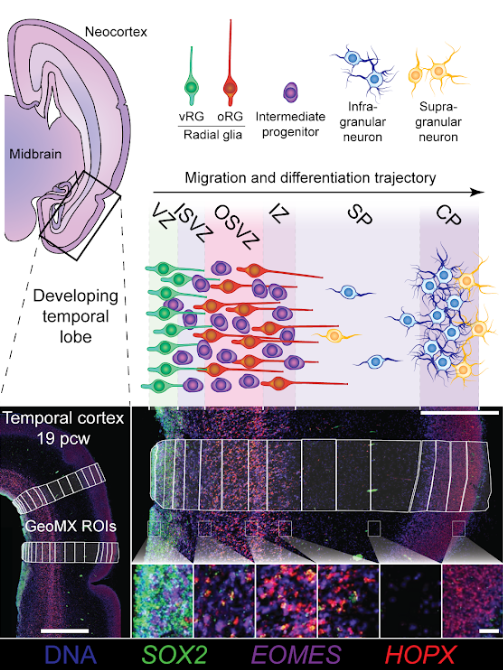
In this notebook we we map fetal brain cell types to regions of interest (ROIs) profiled with the NanostringWTA technology, using a version of our cell2location method recommended for probe based spatial transcriptomics data. This notebook should be read after looking at the main cell2location notebooks.

Load the required modules and configure theano settings:

[1]:

import sys,os
import pickle
import anndata
import pandas as pd
import numpy as np
import matplotlib.pyplot as plt
import scanpy as sc
from IPython.display import Image
data_type = 'float32'
os.environ["THEANO_FLAGS"] = 'device=cuda,floatX=' + data_type + ',force_device=True' + ',dnn.enabled=False'
import cell2location

Can not use cuDNN on context None: Disabled by dnn.enabled flag
Mapped name None to device cuda: Tesla V100-SXM2-32GB (0000:89:00.0)

[6]:

# Download data:
os.mkdir('./data')
os.system('cd ./data && wget https://cell2location.cog.sanger.ac.uk/nanostringWTA/nanostringWTA_fetailBrain_AnnData_smallestExample.p')
os.system('cd ./data && wget https://cell2location.cog.sanger.ac.uk/nanostringWTA/polioudakis2019_meanExpressionProfiles.csv')

[6]:

Load a data:

[7]:

adata_wta = pickle.load(open("data/nanostringWTA_fetailBrain_AnnData_smallestExample.p", "rb" ))

In this NanostringWTA run we profiled 288 regions of interest (ROIs) spanning the full depth of the cortex and at both 19pcw and 14pcw. An example is shown in the image below, together with the cell types we expect in each region:

[8]:

Image(filename='../images/GeometricROIs.PNG')

[8]:

../_images/notebooks_cell2location_for_NanostringWTA_7_0.png

Here we load an existing matrix of average gene expression profiles for each cell type expected in our nanostringWTA data (taken from the single-cell RNAseq study Polioudakis et al., Neuron, 2019):

[11]:

meanExpression_sc = pd.read_csv("data/polioudakis2019_meanExpressionProfiles.csv", index_col=0)

We need seperate gene probes and negative probes and if available we can also supply nuclei counts. We initialize all of those here:

[12]:

counts_negativeProbes = np.asarray(adata_wta[:,np.array(adata_wta.var_names =='NegProbe-WTX').squeeze()].X)
counts_nuclei = np.asarray(adata_wta.obs['nuclei']).reshape(len(adata_wta.obs['nuclei']),1)
adata_wta = adata_wta[:,np.array(adata_wta.var_names != 'NegProbe-WTX').squeeze()]

As you can see the nuclei counts and negative probes need to be numpy arrays, but the gene probe counts are supplied as an AnnData object.

[13]:

adata_wta.raw = adata_wta

Run cell2location:

Explanations of the arguments are as follows: ‘model_name = cell2location.models.LocationModelWTA’ > Here we tell cell2location to use the NanostringWTA model, rather than the standard model. ‘use_raw’: False > extract the data from adata_wta.X and not from adata_wta.raw.X ‘Y_data’: counts_negativeProbes > we supply the negative probe information here ‘cell_number_prior’ and ‘cell_number_var_prior’: we supply information about nuclei counts here

[14]:

cell2location.run_c2l.run_cell2location(meanExpression_sc, adata_wta,
        model_name=cell2location.models.LocationModelWTA,
        train_args={'use_raw': False},
        model_kwargs={
        "Y_data" : counts_negativeProbes,
        "cell_number_prior" : {'cells_per_spot': counts_nuclei, 'factors_per_spot': 6, 'combs_per_spot': 3},
        "cell_number_var_prior" : {'cells_mean_var_ratio': 1, 'factors_mean_var_ratio': 1, 'combs_mean_var_ratio': 1}})

### Summarising single cell clusters ###
### Creating model ### - time 0.0 min

WARNING (theano.gof.cmodule): ModuleCache.refresh() Found key without dll in cache, deleting it. /nfs/users/nfs_a/aa16/.theano/compiledir_Linux-4.15--generic-x86_64-with-debian-buster-sid-x86_64-3.7.6-64/tmp17b1kxnq/key.pkl
WARNING (theano.gof.compilelock): Overriding existing lock by dead process '57693' (I am process '49779')

### Analysis name: LocationModelWTA_1experiments_16clusters_288locations_15124genes
### Training model ###

Average Loss = 5.0222e+07: 100%|██████████| 20000/20000 [03:16<00:00, 101.68it/s]
Finished [100%]: Average Loss = 5.0222e+07

[<matplotlib.lines.Line2D object at 0x1506a7fc3f50>]

Average Loss = 5.0222e+07: 100%|██████████| 20000/20000 [03:16<00:00, 101.73it/s]
Finished [100%]: Average Loss = 5.0222e+07

[<matplotlib.lines.Line2D object at 0x150674f14a90>]

/nfs/team283/aa16/software/miniconda3/envs/cellpymc/lib/python3.7/site-packages/cell2location-0.5-py3.7.egg/cell2location/models/base/pymc3_model.py:449: MatplotlibDeprecationWarning: Passing non-integers as three-element position specification is deprecated since 3.3 and will be removed two minor releases later.
  plt.subplot(nrow, ncol, i + 1)
/nfs/team283/aa16/software/miniconda3/envs/cellpymc/lib/python3.7/site-packages/cell2location-0.5-py3.7.egg/cell2location/models/base/pymc3_model.py:450: MatplotlibDeprecationWarning: Adding an axes using the same arguments as a previous axes currently reuses the earlier instance.  In a future version, a new instance will always be created and returned.  Meanwhile, this warning can be suppressed, and the future behavior ensured, by passing a unique label to each axes instance.
  plt.subplot(np.ceil(n_plots / ncol), ncol, i + 1)

### Sampling posterior ### - time 7.79 min

... storing 'panel' as categorical
... storing 'construct' as categorical
... storing 'instrument_type' as categorical
... storing 'read_pattern' as categorical
... storing 'ngs_prep' as categorical
... storing 'pcr_primer_plate' as categorical
... storing 'pcr_primer_well' as categorical
... storing 'Index 1' as categorical
... storing 'Barcode 1' as categorical
... storing 'Index 2' as categorical
... storing '\tBarcode 2' as categorical
... storing 'segment_type' as categorical
... storing 'segment' as categorical
... storing 'aoi' as categorical
... storing 'dsp_date' as categorical
... storing 'dsp_well' as categorical
... storing 'slide' as categorical
... storing 'human_sample_ID' as categorical
... storing 'slide_barcode' as categorical
... storing 'age' as categorical
... storing 'source_ID' as categorical
... storing 'Sanger_sampleID' as categorical

### Saving results ###

... storing 'AOI_type' as categorical
... storing 'Region' as categorical
... storing 'Plate' as categorical
... storing 'sample' as categorical

### Ploting results ###
[<matplotlib.lines.Line2D object at 0x1506745ffa50>]
[<matplotlib.lines.Line2D object at 0x150674602410>]
[<matplotlib.lines.Line2D object at 0x150674551090>]
[<matplotlib.lines.Line2D object at 0x1506746c5110>]
### Plotting posterior of W / cell locations ###
Some error in plotting with scanpy or `cell2location.plt.plot_factor_spatial()`
 KeyError('coords')
### Done ### - time 8.25 min

[14]:

{'sc_obs':                       End     ExDp1     ExDp2       ExM     ExM-U       ExN  \
 TSPAN6           0.088608  0.016184  0.000000  0.048768  0.026196  0.036418
 DPM1             0.059072  0.130456  0.078313  0.100489  0.101936  0.079940
 SCYL3            0.012658  0.022070  0.030120  0.021890  0.029043  0.014707
 C1orf112         0.000000  0.009809  0.012048  0.006516  0.009112  0.005103
 FGR              0.016878  0.000490  0.000000  0.000000  0.000000  0.000000
 ...                   ...       ...       ...       ...       ...       ...
 ENSG00000276144  0.000000  0.000000  0.000000  0.000102  0.000569  0.000100
 SNORD114-7       0.000000  0.000000  0.006024  0.000000  0.000000  0.000000
 ZNF965P          0.000000  0.000000  0.000000  0.000102  0.000000  0.000100
 GOLGA8K          0.000000  0.000981  0.000000  0.000102  0.000000  0.000000
 GOLGA8J          0.000000  0.000000  0.000000  0.000000  0.000000  0.000200

                     InCGE     InMGE        IP       Mic       OPC       oRG  \
 TSPAN6           0.012552  0.011144  0.089767  0.000000  0.075163  0.241299
 DPM1             0.085077  0.073900  0.113953  0.062500  0.183007  0.169374
 SCYL3            0.013947  0.017009  0.019535  0.000000  0.049020  0.035576
 C1orf112         0.007671  0.004692  0.007907  0.020833  0.026144  0.028616
 FGR              0.000000  0.000587  0.000000  0.000000  0.000000  0.000000
 ...                   ...       ...       ...       ...       ...       ...
 ENSG00000276144  0.000000  0.000000  0.000000  0.000000  0.000000  0.000000
 SNORD114-7       0.000000  0.000000  0.000000  0.000000  0.000000  0.000000
 ZNF965P          0.000000  0.000000  0.000000  0.000000  0.000000  0.000000
 GOLGA8K          0.000000  0.000000  0.000000  0.000000  0.000000  0.000773
 GOLGA8J          0.000000  0.000000  0.000000  0.000000  0.000000  0.000000

                       Per     PgG2M       PgS       vRG
 TSPAN6           0.043860  0.162590  0.125000  0.228659
 DPM1             0.157895  0.276259  0.270292  0.155488
 SCYL3            0.026316  0.021583  0.034903  0.034553
 C1orf112         0.017544  0.046043  0.051136  0.009146
 FGR              0.000000  0.000000  0.000000  0.000000
 ...                   ...       ...       ...       ...
 ENSG00000276144  0.000000  0.000000  0.000000  0.000000
 SNORD114-7       0.000000  0.001439  0.000000  0.000000
 ZNF965P          0.000000  0.000000  0.000000  0.000000
 GOLGA8K          0.000000  0.000000  0.000000  0.000000
 GOLGA8J          0.000000  0.000000  0.000812  0.000000

 [35543 rows x 16 columns],
 'model_name': cell2location.models.LocationModelWTA.LocationModelWTA,
 'summ_sc_data_args': {'cluster_col': 'annotation_1',
  'which_genes': 'intersect',
  'selection': 'cluster_specificity',
  'select_n': 5000,
  'select_n_AutoGeneS': 1000,
  'selection_specificity': 0.07,
  'cluster_markers_kwargs': {}},
 'train_args': {'mode': 'normal',
  'use_raw': False,
  'data_type': 'float32',
  'n_iter': 20000,
  'learning_rate': 0.005,
  'total_grad_norm_constraint': 200,
  'method': 'advi',
  'sample_prior': False,
  'n_prior_samples': 10,
  'n_restarts': 2,
  'n_type': 'restart',
  'tracking_every': 1000,
  'tracking_n_samples': 50,
  'readable_var_name_col': None,
  'sample_name_col': 'sample',
  'fact_names': None,
  'minibatch_size': None},
 'posterior_args': {'n_samples': 1000,
  'evaluate_stability_align': False,
  'mean_field_slot': 'init_1'},
 'export_args': {'path': './results',
  'plot_extension': 'png',
  'scanpy_plot_vmax': 'p99.2',
  'scanpy_plot_size': 1.3,
  'save_model': False,
  'save_spatial_plots': True,
  'run_name_suffix': '',
  'export_q05': True,
  'export_mean': False,
  'scanpy_coords_name': 'coords',
  'img_key': 'hires'},
 'run_name': 'LocationModelWTA_1experiments_16clusters_288locations_15124genes',
 'run_time': '8.23 min',
 'mod': <cell2location.models.LocationModelWTA.LocationModelWTA at 0x1506fb6ba690>}

An anndata object that has the cell2location results included is saved and can be used for further analysis, as in standard cell2location:

[2]:

adata_c2l = sc.read_h5ad('resultsLocationModelWTA_1experiments_16clusters_288locations_15124genes/sp.h5ad')

[19]:

adata_c2l.obs.loc[:,['mean_spot_factors' in c for c in adata_c2l.obs.columns]]

[19]:

	mean_spot_factorsEnd	mean_spot_factorsExDp1	mean_spot_factorsExDp2	mean_spot_factorsExM	mean_spot_factorsExM-U	mean_spot_factorsExN	mean_spot_factorsInCGE	mean_spot_factorsInMGE	mean_spot_factorsIP	mean_spot_factorsMic	mean_spot_factorsOPC	mean_spot_factorsoRG	mean_spot_factorsPer	mean_spot_factorsPgG2M	mean_spot_factorsPgS	mean_spot_factorsvRG
0	0.084664	0.189308	0.029214	0.416038	2.362057	11.295574	16.262985	7.932218	41.685520	0.742107	0.223058	0.236820	0.672671	3.205585	12.560131	13.601164
1	21.419926	7.724943	6.721371	0.333573	1.066788	0.770727	48.214741	42.975559	70.506340	8.807492	14.691536	521.252258	13.545335	49.975002	10.506875	487.543640
2	39.654678	19.112091	12.900160	21.181322	16.252541	434.558960	340.707214	129.871735	349.923279	25.703894	21.041853	290.028412	20.612944	57.256882	78.789604	84.983528
3	51.285645	8.662683	15.469158	3.503401	14.038322	896.294128	295.430023	152.729813	521.571167	30.252962	31.993980	456.301239	28.588427	86.054306	129.775269	132.642563
4	25.595606	23.515396	48.510769	188.190826	26.642292	499.026337	80.059036	41.910606	116.886253	13.355888	19.981899	98.308342	17.650003	32.258457	86.578354	41.804352
...	...	...	...	...	...	...	...	...	...	...	...	...	...	...	...	...
283	0.028876	0.035472	0.006267	0.040910	0.031838	0.053754	0.025631	0.023575	0.035022	0.027488	0.013950	0.017187	0.010829	0.009468	0.020645	0.021043
284	0.043387	0.037010	0.013416	0.059270	0.047244	0.050790	0.043571	0.042204	0.043056	0.029641	0.020657	0.024773	0.011805	0.069313	0.048026	0.035278
285	0.020425	0.013803	0.007025	0.006270	0.005928	0.015476	0.014805	0.012487	0.010647	0.018965	0.005501	0.009071	0.007763	0.003181	0.005728	0.010816
286	0.015542	0.010659	0.007960	0.008583	0.007580	0.010384	0.013900	0.010033	0.013732	0.011912	0.007894	0.009918	0.004368	0.002940	0.005661	0.007249
287	0.012233	0.011973	0.004245	0.006267	0.014237	0.012098	0.014255	0.018113	0.009493	0.012822	0.006665	0.007838	0.003509	0.004466	0.008221	0.009287

288 rows × 16 columns

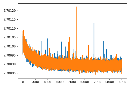
We can also plot the same QC metrics as in standard cell2location:

[21]:

from IPython.display import Image
Image(filename='resultsLocationModelWTA_1experiments_16clusters_288locations_15124genes/plots/training_history_without_first_20perc.png',
      width=400)

[21]:

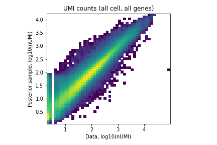
../_images/notebooks_cell2location_for_NanostringWTA_21_0.png

[22]:

Image(filename='resultsLocationModelWTA_1experiments_16clusters_288locations_15124genes/plots/data_vs_posterior_mean.png',
      width=400)

[22]:

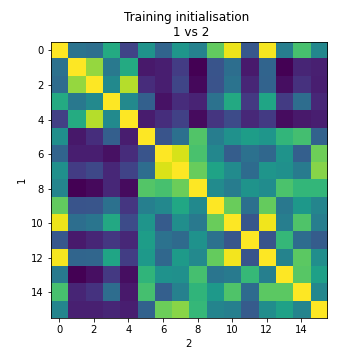
../_images/notebooks_cell2location_for_NanostringWTA_22_0.png

[23]:

Image(filename='resultsLocationModelWTA_1experiments_16clusters_288locations_15124genes/plots/evaluate_stability.png',
      width=400)

[23]:

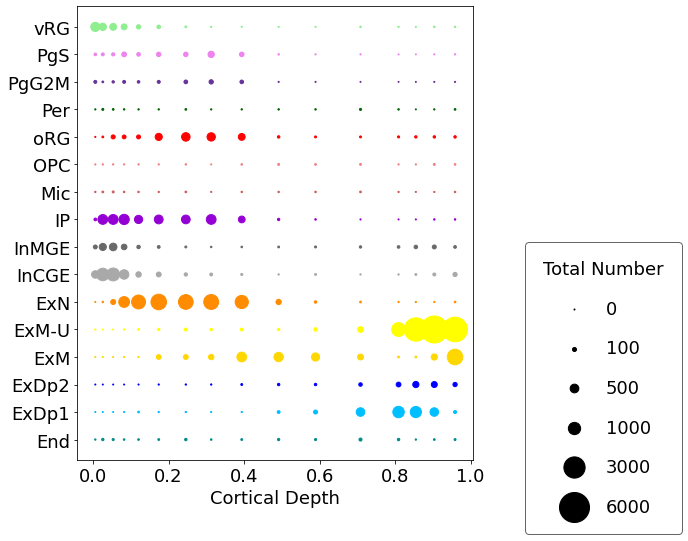
../_images/notebooks_cell2location_for_NanostringWTA_23_0.png

Finally we have this method to plot cell type abundance in 1D across our coordinate of interest (cortical depth):

It makes most sense to plot a subset, for example on one 19pcw slide at one position:

[3]:

colourCode = {'SPN': 'salmon', 'End': 'darkcyan', 'ExDp1': 'deepskyblue', 'ExDp2': 'blue', 'ExM': 'gold', 'ExM-U': 'yellow',
              'ExN': 'darkorange', 'InCGE': 'darkgrey', 'InMGE': 'dimgray', 'IP': 'darkviolet',
              'Mic': 'indianred', 'OPC': 'lightcoral', 'oRG': 'red', 'Per': 'darkgreen',
              'PgG2M': 'rebeccapurple', 'PgS': 'violet', 'vRG': 'lightgreen'}

[4]:

subset_19pcw = [adata_c2l.obs['slide'].iloc[i] == '00MU' and
         adata_c2l.obs['Radial_position'].iloc[i] == 2 for i in range(len(adata_c2l.obs['Radial_position']))]

[5]:

cell2location.plt.plot_absolute_abundances_1D(adata_c2l, subset = subset_19pcw, saving = False,
                               scaling = 0.15, power = 1, pws = [0,0,100,500,1000,3000,6000], figureSize = (12,8),
                               dimName = 'VCDepth', xlab = 'Cortical Depth', colourCode = colourCode)

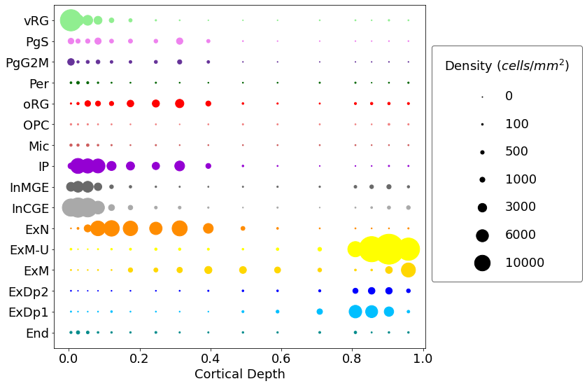
../_images/notebooks_cell2location_for_NanostringWTA_28_0.png

You can also plot density rather than total numbers:

[7]:

cell2location.plt.plot_density_1D(adata_c2l, subset = subset_19pcw, saving = False,
                               scaling = 0.05, power = 1, pws = [0,0,100,500,1000,3000,6000,10000], figureSize = (12,8),
                               dimName = 'VCDepth', areaName = 'roi_dimension', xlab = 'Cortical Depth',
                colourCode = colourCode)

../_images/notebooks_cell2location_for_NanostringWTA_30_0.png

[ ]: